Autoencoders and latent space fragmentation – VII – face images from statistical z-points close to the latent space region of CelebA

I continue with my analysis of the z-point and latent vector distribution a trained Autoencoder creates in its latent space for CelebA images. These images show human faces. To make the Autoencoder produce new face images from statistically generated latent vectors is a problem. See some previous posts in this series for reasons.

Autoencoders and latent space fragmentation – I – Encoder, Decoder, latent space
Autoencoders and latent space fragmentation – II – number distributions of latent vector components
Autoencoders and latent space fragmentation – III – correlations of latent vector components
Autoencoders and latent space fragmentation – IV – CelebA and statistical vector distributions in the surroundings of the latent space origin
Autoencoders and latent space fragmentation – V – reconstruction of human face images from simple statistical z-point-distributions?

These problems are critical for a generative usage of standard Autoencoders. Generative tasks in Machine Learning very often depend on a clear and understandable structure of the latent space regions an Encoder/Decoder pair uses. In general we would like to create statistical latent vectors such that a reasonable object creation (here: image creation) is guaranteed. In the last post

Autoencoders and latent space fragmentation – VI – image creation from z-points along paths in selected coordinate planes of the latent space

we saw that we at least get some clear face features when we make use of some basic information about the shape and location of the z-point distribution for the images the AE was trained with. This distribution is specific for an Autoencoder, the image set used and details of the training run. In our case the z-point distribution could be analyzed by rather simple methods after the training of an AE with CelebA images had been concluded. The number distribution curves per vector component revealed value limits per latent vector component. The core of the z-point distribution itself appeared to occupy a single and rather compact sub-volume inside the latent space. (The exact properties depend on the AE’s layer structure and the training run.) Of the N=256 dimensions of our latent space only a few determined the off-origin position of the center of the z-point distribution’s core. This multidimensional core had an overall ellipsoidal shape. We could see this both from the Gaussian like number distributions for the components and more directly from projections onto 2-dimensional coordinate planes. (We will have a closer look at these properties which indicate a multivariate normal distribution in forthcoming posts.)

As long as we kept the statistical values for artificial latent vector components within the value ranges set by the distribution’s core our chances that the AE’s Decoder produced images with new and clearly visible faces rose significantly. So far we have only used z-points along defined paths crossing the distributions core. In this post I will vary the components of our statistically created latent vectors a bit more freely. This will again show us that correlations of the vector components are important.

Constant probability for each component value within a component specific interval

In the first posts of this series I naively created statistical latent vectors from a common value range for the components. We saw this was an inadequate approach – both for general mathematical and for problem specific reasons. The following code snippets shows an approach which takes into account value ranges coming from the Gaussian-like distributions for the individual components of the latent vectors for CelebA. The arrays “ay_mu_comp” and “ay_mu_hw” have the following meaning:

  • ay_mu_comp: Component values of a latent vector pointing to the center of the CelebA related z-point distribution
  • ay_mu_hw: Half-width of the Gaussian like number distribution for the component specific values
num_per_row  = 7
num_rows     = 3
num_examples = num_per_row * num_rows

fact = 1.0

# Get component specific value ranges into an array 
li_b = []
for j in range(0, z_dim):  
    add_val = fact*abs(ay_mu_hw[j])
    b_l = ay_mu_comp[j] - add_val
    b_r = ay_mu_comp[j] + add_val
    li_b.append((b_l, b_r))
    
# Statistical latent vectors
ay_stat_zpts = np.zeros( (num_examples, z_dim), dtype=np.float32 )     
for i in range(0, num_examples): 
    for j in range(0, z_dim):
        b_l = li_b[j][0]
        b_r = li_b[j][1]
        val_c = np.random.uniform(b_l, b_r) 
        ay_stat_zpts[i, j] = val_c

# Prediction 
reco_img_stat = AE.decoder.predict(ay_stat_zpts)
# print("Shape of reco_img = ", reco_img_stat.shape)

The main difference is that we take random values from real value intervals defined per component. Within each interval we assume a constant probability density. The factor “fact” controls the width of the value interval we use. A small value covers the vicinity of the center of the CelebA z-point distribution; a larger fact leads to values at the border region of the z-point distribution.

Image results for different value ranges

fact=0.4

fact=0.5

fact=0.6

fact=0.7

fact=0.8

fact=0.9

fact=1.0

Selected individuals

Below you find some individual images created for a variety of statistical vectors. They are ordered by a growing distance from the center of the CelebA related z-point distribution.

Quality? Missing correlations?

The first thing we see is that we get problems for all factors fact. Some images are OK, but others show disturbances and the contrasts of the face against the background are not well defined – even for small factors fact. The reason is that our random selection ignores correlations between the components completely. But we know already that there are major correlations between certain vector components.

For larger values of fact the risk to place a generated latent vector outside the core of the CelebA z-point distribution gets bigger. Still some images interesting face variations.

Obviously, we have no control over the transitions from face to hair and from hair to background. Our suspicion is that micro-correlations of the latent vector components for CelebA images may encode the respective information. To understand this aspect we would have to investigate the vicinity of a z-point a bit more in detail.

Conclusion

We are able to create images with new human faces by using statistical latent vectors whose component values fall into component specific defined real value intervals. We can derive the limits of these value ranges from the real z-point distribution for CelebA images of a trained AE. But again we saw:

One should not ignore major correlations between the component values.

We have to take better care of this point in a future post when we perform a transformation of the coordinate system to align with the main axes of the z-point distribution. But there is another aspect which is interesting, too:

Micro-correlations between latent vector components may determine the transition from faces to complex hair and background-patterns.

We can understand such component dependencies when we assume that the superposition especially of small scale patterns a convolutional Decoder must arrange during image creation is a subtle balancing act. A first step to understand such micro-correlations better could be to have a closer look at the nearest CelebA z-point neighbors of an artificially created latent z-point. If they form some kind of pattern, then maybe we can change the components of our z-point a bit in the right direction?

Or do we have to deal with correlations on a much coarser level? What do the Gaussians and the roughly elliptic form of the core of the z-point distribution for CelebA images really imply? This is the topic of the next post.

Autoencoders and latent space fragmentation – VIII – approximation of the latent vector distribution by a multivariate normal distribution and ellipses


Autoencoders and latent space fragmentation – VI – image creation from z-points along paths in selected coordinate planes of the latent space

It is well known that standard (convolutional) Autoencoders [AEs] cause problems when you want to use them for creative purposes. An example: Creating images with human faces by feeding the Decoder of a suitably trained AE with random latent vectors does not work well. In this series of posts I want to identify the cause of this specific problem. Another objective is to circumvent some of the related obstacles and create reasonably clear images nevertheless. Note that I speak about standard Autoencoders, not Variational Autoencoders or transformer based Encoder/Decoder-systems. For basic concepts, terms and methods see the previous posts:

Autoencoders and latent space fragmentation – I – Encoder, Decoder, latent space
Autoencoders and latent space fragmentation – II – number distributions of latent vector components
Autoencoders and latent space fragmentation – III – correlations of latent vector components
Autoencoders and latent space fragmentation – IV – CelebA and statistical vector distributions in the surroundings of the latent space origin
Autoencoders and latent space fragmentation – V – reconstruction of human face images from simple statistical z-point-distributions?

So far I have demonstrated that randomly generated vectors most often do not hit the relevant regions in the AE’s latent space – if we do not take some data specific precautions. A relevant region is a confined volume which a trained Decoder fills with z-points for its training objects after the training has been completed. z-points and corresponding latent vectors are the result of an encoding process which maps digitized input objects into the latent space. Depending on the data objects we may get multiple relevant regions or just one compact region. In the case of a convolutional AE which I had trained with the CelebA dataset of human face images I found single region with a rather compact core.

In this post I want to create statistical latent vectors whose end-points are located inside the relevant region for CelebA images. Then I will create images from such latent vectors with the help of the AE’s Decoder. My hope is to get at least some images with clearly visible human faces. The basic idea behind this experiment is that the most important features of human faces are encoded by a few dominant vector components defining the overall position and shape of the multidimensional z-point region for CelebA images. We will see that the theory is indeed valid: Here is a first example for a vector pointing to an outer area of the core region for CelebA images in the latent space:

Our AE is a convolutional one. The number of latent space dimensions N was chosen to be N=256.
Note: We are NOT using a Variational Autoencoder, but a simple standard Autoencoder. The AE’s properties were discussed in previous posts.

What have we found out so far?

The Encoder of the convolutional AE, which I had trained with the CelebA dataset, mapped the human face images into a compact region of the latent space. The core of the created z-point distribution was located within or very close to a tiny hyper-volume of the latent space spanned by only a few coordinate axes. The confined multi-dimensional volume occupied by most of the z-points had an overall ellipsoidal shape with major extensions along a few main axes. We saw that some of the coordinates of the CelebA z-points and the components of the corresponding latent vectors were strongly correlated. In addition the value range of each of the latent vector components had specific individual limits – confining the angles and lengths of the vectors for CelebA. Therefore we had to conclude:

Whenever we base our method to create statistical vectors on the assumptions

  • that one can treat the vector components as independent statistical variables
  • that one can assign statistical values to the components from a common real value interval

the vectors will almost certainly not point to the relevant region. In addition one has to take into account unexpected mathematical properties of statistical vector distributions in high dimensional spaces. See the previous posts for more details. Indeed we could show that such a vector generation method missed the CelebA region.

Objective of this post

In this post I want to use some of the knowledge which we have gathered about the latent vector distribution for CelebA images. We shall use a very simple approach to probe the image reconstruction abilities of the Decoder for a defined variety of z-points:

We restrict the vectors’ component values such that most of the vectors point to the region formed by the bulk of CelebA z-points. To achieve this we define straight line segments which cross the ellipsoidal region of CelebA z-points. This is possible due to the known value intervals which we have identified for each of the components in a previous post. Then we place some artificial z-points onto our line segments. At least some of these z-points will fall into the relevant CelebA region. We then let the Decoder reconstruct images for the latent vectors corresponding to these z-points.

In some cases our paths will even respect some major component correlations, but for some paths I will explicitly disregard such correlations. Nevertheless our rather simple restrictions imposed on the vector-component values will already enable us to produce images with clearly recognizable face features.

Among other things our results confirm the idea that the real pixel correlations for basic face features are represented by relatively narrow limits for the angles and lengths of respective latent vectors. The extension and shape of the bulk region of CelebA z-points is defined by only a few latent vector components. These components apparently encode a prescription for the (convolutional) Decoder to create face features by a superposition of some elementary patterns extracted during the AE’s training.

A path from the latent space origin to the center of the relevant z-point region

How do we restrict latent vectors to the required value ranges? In the 2nd post we have seen that the number distribution curve for the values of each of the latent vector components was very similar to a Gaussian. We have identified the mean value and average value range for each component by analyzing its specific distribution curve. The mean values gave us the coordinates of the center of the relevant latent space region. In addition we, of course, know the coordinates of the origin of the latent space. So, for a first test, let us create a multi-dimensional line segment between the origin and the center of the CelebA z-point distribution. And let the A’s Decoder create images for latent vectors pointing to some intermediate z-points along this path.

The following plots show orthogonal projections of 5000 CelebA z-points (in blue) onto some 2-dimensional planes spanned by two selected coordinate axes. The yellow dot indicates the origin. The orange dot the center of the z-point distribution. Red dots indicate coordinates of points along the straight path between the origin and the distribution center.

Please, take note of the different scales on the x- and y-axes. Some distributions are much more elongated than the scaled images show. That some paths appear shorter than others is due to the projection of the diagonal line through the multi-dimensional space onto planes which are differently oriented with respect to this line. A simple 3D analog should make this clear. Some small wiggles in the positions of the red dots are due to resolution problems of the plot on the browser interface. We also see a reflection of the fact that the origin is located in a border region of the bulk.

Below you see a plot which shows the path in higher resolution (projected onto a particular plane):

Again: Take note of the different axis scales. The blue dot distribution is much more stretched in C1-direction than it appears in the plot.

Ok, now we have a multidimensional path and six well defined latent vectors for the end and intermediate points on this path. So let us provide these vectors as input to the our AE’s Decoder. The resulting images look like:

Success! Images in the surroundings of the center show a clearly visible face. And we also see: The average face at the center of the z-point distribution is female – at least according to the CelebA dataset. 🙂 However: In the vicinity of the origin of the latent space we get no images with reasonable face features.

Images along a path within a selected coordinate plane for two dominant vector components

I choose a different path within the plane spanned by the coordinates axes 151 and 195 now. This is depicted in the plot below:

A look into the second post shows you that the components 151, 195 were members of the group of dominant components. Those were components for which the number distribution showed a mean value at some distance from the origin of the latent space and also had a half-width bigger than 1.0 (as most of the other components). The images reconstructed by the Decoder from the latent vectors are:

Hey, we get some variation – as expected. Now, let us rotate the path in the plane:

Not so much of a difference. But we have learned that a variation of some vector component values within the allowed range of values may give us already some major variation in the faces’ expressions.

Images for other coordinate planes

The following images show the variations for paths in other coordinate planes. All of the paths have in common that they pass the center of the CelebA bulk region. For the first 4 examples I have kept the path within the core region of CelebA z-points. The last images show images for paths with z-points at the core’s border regions or a bit outside of it.

Plane axes: 5, 8

Plane axes: 17, 180

Plane axes: 44, 111

Plane axes: 55, 56

Plane axes: 15, 242

Plane axes: 58 202

Plane axes: 68, 178

Plane axes: 177, 202

Plane axes: 180, 242

The images for z-points farther away from the bulk’s center give you more interesting variations. But obviously in the outer areas of the CelebA region correlations between the latent vector components get more important when we want to avoid irregular and unrealistic disturbances. All in all we also get the impression that a much more subtle correlation of component values is a key for the reproduction of realistic transitions for the hairdos presented in the CelebA images and the transition to some realistic background patterns. The components of our latent vectors are still too uncorrelated for such details and an appropriate superposition of micro-patterns in the images created by the Decoder.

Conclusion

This blog shows that we do not need a Variational Autoencoder to produce images with recognizable human faces from statistical latent vectors. We can get image reproductions with varying face features also from the Decoder of a standard convolutional Autoencoder. A basic requirement seems to be that we keep the vector components within reasonable value intervals. The valid component specific value ranges are defined by the shape of the compact hyper-volume, which an AE’s Encoder fills with z-points for its training objects. So we need to construct statistical latent vectors which point to this specific sub-region of the latent space. Vectors with arbitrary components will almost certainly miss this region and give no interpretable image content.

In this post we have looked at vectors defining z-points along specific line segments in the latent space. Some of the paths were explicitly kept within the inner core regions of the z-point-distribution for CelebA images. From these z-points the most important face features were clearly reconstructed. But we also saw that some micro-correlations of the latent vector components seem to control the appearance of the background and the transition from the face to hair and from the hair to the background-environment.

I have not yet looked at line segments which do not cross the center of the bulk of the z-point distribution for CelebA images in the latent space. But in the next post

Autoencoders and latent space fragmentation – VII – face images from statistical z-points close to the latent space region of CelebA

I first want to look at z-points for which we relatively freely vary the component values within ranges given by the respective number distributions.


Autoencoders and latent space fragmentation – IV – CelebA and statistical vector distributions in the surroundings of the latent space origin

I continue with my investigation of the z-point- and latent vector distribution which a convolutional Autoencoder [AE] creates in its latent space for CelebA images. Such images show human faces – and our objective is to find out whether we can force the AE’s Decoder to create human face images from artificially generated and statistically distributed z-points in the latent space. E.g. for creative tasks – without using a Variational Autoencoder.

The first posts of this series

Autoencoders and latent space fragmentation – I – Encoder, Decoder, latent space
Autoencoders and latent space fragmentation – II – number distributions of latent vector components
Autoencoders and latent space fragmentation – III – correlations of latent vector components

have revealed that the multi-dimensional volume region filled with z-points for CelebA images is rather small and has an ellipsoidal shape. The region is extended in the direction of a few main axes. Its center is located at some distance from the origin of the latent space. Its position is rather close to or within a hyper-volume of the latent space spanned by a few axes, only. The origin of the latent space is instead located close to the border of the bulk region of CelebA z-points.

We have also found out that artificially created z-points may miss the region of the CelebA z-points. In particular when we generate respective vectors under the assumption that the vector components are independent variables and can be filled with values obeying a constant probability distribution within a real value interval [-b, b]. See the second post for links to a study of the mathematical properties of such artificial vector distributions. We saw that the radii of the artificial vectors only match those of CelebA vectors if we choose 1.0 < b < 2.0. An optimal value appeared to be b = 1.5. This means that the created statistical vectors would have positions relatively close to the origin. We had hoped that such artificial vectors overlap at least in parts with the latent vector distribution for CelebA. Such an overlap may be required to get a reconstruction of images with clearly visible human faces.

In this post I, therefore, have a look at the surroundings of the latent space origin. We focus on projections of the neighboring z-points onto planes formed by selected latent vector components. We choose these components such that the border position of the origin with respect to the volume occupied by the bulk of CelebA z-points becomes clear. We afterward look at real and artificial z-points close to a slice of the multi-dimensional latent space volume. The vectors to the z-points in this slice fulfill the following condition: All components x_j, with the exception of two selected ones, have values x_j < 1.5. This will reduce projection effects with respect to the selected projection plane. The results will show us that many of the artificial z-points unfortunately fall into empty regions (voids). It is sufficient to show this for some selected coordinate pairs. The latent space of our AE has N=256 dimensions.

Position of the origin with respect to the CelebA z-point distribution

First I want to remind you of the border position of the latent space’s origin with respect to the bulk of the CelebA z-point-distribution. The following plots show again 5000 randomly selected z-points corresponding to latent vectors for CelebA images (blue points). The yellow point marks the origin of the latent space. The red dots correspond to 10 artificially created z-points for b = 1.5. The individual plots correspond to selected pairs of vector components and planes spanned by respective axes.

That the center of the distribution appears extremely densely populated is a bit due to the chosen diameter of the blue points. When interpreting these plots, please note: We are looking at orthogonal projections. Therefore we always have to take into account projection effects.

A closer look at the environment of the latent space’s origin

The following plot shows the environment of the origin with a higher resolution for our 5600 z-points. Despite the fact that this is a projection of many points onto the selected plane we get a first impression that CelebA z-point distribution is not really a homogeneous one – although being a relatively dense one around the center of the ellipsoidal bulk distribution.

Some of our artificial z-points seem in both cases to mix with the CelebA z-points. Below I want to show that this is a projection effect, only.

The surroundings of the origin in a flat cuboid

In the second post of this series we had derived that a parameter b = 1.5 is optimal to get the right vector length of our artificial statistical vectors to match the length of the latent CelebA vectors. Therefore, I have reduced the amount of CelebA z-points by imposing the following conditions on the components x_j:

-1.5 ≤   x_j   ≤ 1.5,    for all j in [0, 256], with the exception of two selected values j = j1 or j = j2

I.e. we look at CelebA z-points close to the plane defined by the axes corresponding to our specially selected vector components x_j1 and x_j2. Thus we get rid of projection effects from any points outside the multi-dimensional slice. We only get projections from points inside our multi-dimensional slice, which contains the cube defined by a side-length -1.5 ≤ x_j ≤ +1.5 around the origin. Our statistically generated vectors have end-points inside this multi-dimensional cube. The result is:

Ooops, only two out of our 5000 CelebA points are present in the slice region, which I also have populated with 200 artificial z-points. So, clearly this is not a region which the AE’s Encoder fills densely for CelebA images.

Even for 80,000 CelebA z-points the situation does not improve so much. Only 56 latent CelebA vectors point to our region.

Most of the artificially created z-points (in red) thus come to fall into empty volume regions – regions not used by CelebA z-points. This already diminishes our chances to reconstruct reasonable human face images by our artificial distribution of latent vectors.

Situation for a second and a third plane

Can we reproduce this also for other component pairs? Yes, indeed, e.g. for the pair (177, 242):

For 5000 CelebA z-points:

Only one out of 5000 CelebA vectors points to the relevant slice:

For 80,000 images 39 regular CelebA z-points survive, only. I skip the respective image.

Vector components (30, 118)
Another interesting pair of components and respective coordinate axes is (30, 118):

And for our slice we get:

From 80,000 points only around 70 are located in our slice of the multidimensional space:

Vector components (118, 156)
For the pair (118, 156) the respective plots are:

We see some overlaps between the artificially created points and the CelebA z-points. However, you should keep in mind that the probability that an artificial point falls into a void in the multi-dimensional space gets bigger with every individual component value putting the point outside the CelebA bulk region. And: Our “overlaps” are still the result of a (significantly reduced) projection effect. Furthermore, the plots do not distinguish the components of an individual point from those of other points. If one component shows an overlap with CelebA points, another component for the same point may not. And one component is enough to determine a position outside the bulk.

Radii of the artificially created z-points

When rating probabilities of our artificially created z-points to hit a region populated by CelebA z-points you should also remember that our artificially created points fall into a rather narrow spherical shell for so many dimensions as our latent space has. See the second post of this series for this phenomenon.

Conclusion

What have we learned? The second post in this series gave us hope that at least some of the artificially created z-points (based on independent component values taken with a constant probability from a common value interval) would get a position within the confined region populated by the real CelebA z-points. A closer look, however, showed us that the origin of the latent space resides within a border-region of the ellipsoidal bulk of the multi-dimensional CelebA z-point distribution. Only very few CelebA z-points are found in this border region and within slices close to selected coordinate planes.

What does this mean? The chances that most of the artificially created z-points for b = 1.5 will fall into a void not used by the AE’s Decoder for CelebA images is much bigger than we originally may have thought. In addition our statistical points only populate a spherical shell within a multi-dimensional cube around the origin of the latent space with a side length of 2b. Even if we compensate this effect by generating vectors for different b-values we do not gain much. This raises the fundamental question whether a method that generates statistical z-points via independent component values is a reasonable choice for our objective to reconstruct human face images.

In the next post

Autoencoders and latent space fragmentation – V – reconstruction of human face images from simple statistical z-point-distributions?

I will show that the results of such reconstruction efforts are indeed frustrating. As a consequence I will discuss how we could simply adjust our generating method to the real distribution of latent vectors for CelebA images.


Autoencoders and latent space fragmentation – III – correlations of latent vector components

The topics of this post series are

  • convolutional Autoencoders,
  • images of human faces, provided by the CelebA dataset
  • and related data point and vector distributions in the AEs’ latent spaces.

In the first post

Autoencoders and latent space fragmentation – I – Encoder, Decoder, latent space

I have repeated some basics about the representation of images by vectors. An image corresponds e.g. to a vector in a feature space with orthogonal axes for all individual pixel values. An AE’s Encoder compresses and encodes the image information in form of a vector in the AE’s latent space. This space has many, but significantly fewer dimensions than the original feature space. The end-points of latent vectors are so called z-points in the latent space. We can plot their positions with respect to two coordinate axes in the plane spanned by these axes. The positions reflect the respective vector component values and are the result of an orthogonal projection of the z-points onto this plane. In the second post

Autoencoders and latent space fragmentation – II – number distributions of latent vector components

I have discussed that the length and orientation of a latent vector correspond to a recipe for a constructive process of The AE’s (convolutional) Decoder: The vector component values tell the Decoder how to build a superposition of elementary patterns to reconstruct an image in the original feature space. The fundamental patterns detected by the convolutional AE layers in images of the same class of objects reflect typical pixel correlations. Therefore the resulting latent vectors should not vary arbitrarily in their orientation and length.

By an analysis of the component values of the latent vectors for many CelebA images we could explicitly show that such vectors indeed have end points within a small coherent, confined and ellipsoidal region in the latent space. The number distributions of the vectors’ component values are very similar to Gaussian functions. Most of them with a small standard deviation around a central mean value very close to zero. But we also found a few dominant components with a wider value spread and a central average value different from zero. The center of the latent space region for CelebA images thus lies at some distance from the origin of the latent space’s coordinate system. The center is located close to or within a region spanned by only a few coordinate axes. The Gaussians define a multidimensional ellipsoidal volume with major anisotropic extensions only along a few primary axes.

In addition we studied artificial statistical vector distributions which we created with the help of a constant probability distribution for the values of each of the vector components. We found that the resulting z-points of such vectors most often are not located inside the small ellipsoidal region marked by the latent vectors for the CelebA dataset. Due to the mathematical properties of this kind of artificial statistical vectors only rather small parameter values 1.0 ≤ b ≤ 2.0 for the interval [-b, b], from which we pick all the the component values, allow for vectors with at least the right length. However, whether the orientations of such artificial vectors fit the real CelebA vector distribution also depends on possible correlations of the components.

In this post I will show you that there indeed are significant correlations between the components of latent vectors for CelebA images. The correlations are most significant for those components which determine the location of the center of the z-point distribution and the orientation of the main axes of the z-point region for CelebA images. Therefore, a method for statistical vector creation which explicitly treats the vector components as statistically independent properties may fail to cover the interesting latent space region.

Normalized correlation coefficient matrix

When we have N variables (X_1, x_2, … x_n) and M parallel observations for the variable values then we can determine possible correlations by calculating the so called covariance matrix with elements Cij. A normalized version of this matrix provides the so called “Pearson product-moment correlation coefficients” with values in the range [0.0, 1.0]. Values close to 1.0 indicate a significant correlation of the variables x_i and x_j. For more information see e.g. the following links to the documentation on Numpy’s versions for the calculation of the (normalized) covariance matrix from an array containing the observations in an ordered matrix form: “numpy.cov” and to “numpy.corrcoef“.

So what are the “variables” and “observations” in our case?

Latent vectors and their components

In the last post we have calculated the latent vectors that a trained convolutional AE produces for a 170,000 images of the CelebA dataset. As we chose the number N of dimensions of the latent space to be N=256 each of the latent vectors had 256 components. We can interpret the 256 components as our “variables” and the latent vectors themselves as “observations”. An array containing M rows for individual vectors and N columns for the component values can thus be used as input for Numpy’s algorithm to calculate the normalized correlation coefficients.

When you try to perform the actual calculations you will soon detect that determining the covariance values based on a statistics for all of the 170,000 latent vectors which we created for CelebA images requires an enormous amount of RAM with growing M. So, we have to chose M << 170,000. In the calculations below I took M = 5000 statistically selected vectors out of my 170,000 training vectors.

Some special latent vector components

Before I give you the Pearson coefficients I want to remind you of some special components of the CelebA latent vectors. I had called these components the dominant ones as they had either relatively large absolute mean values or a relatively large half-width. The indices of these components, the related mean values mu and half-widths hw are listed below for a AE with filter numbers in the Encoder’s and Decoder’s 4 convolutional layers given by (64, 64, 128, 128) and (128, 128, 64, 64), respectively:

 15   mu : -0.25 :: hw:  1.5
 16   mu :  0.5  :: hw:  1.125
 56   mu :  0.0  :: hw:  1.625
 58   mu :  0.25 :: hw:  2.125
 66   mu :  0.25 :: hw:  1.5
 68   mu :  0.0  :: hw:  2.0
110   mu :  0.5  :: hw:  1.875
118   mu :  2.25 :: hw:  2.25
151   mu :  1.5  :: hw:  4.125
177   mu : -1.0  :: hw:  2.25
178   mu :  0.5  :: hw:  1.875
180   mu : -0.25 :: hw:  1.5
188   mu :  0.25 :: hw:  1.75
195   mu : -1.5  :: hw:  2.0
202   mu : -0.5  :: hw:  2.25
204   mu : -0.5  :: hw:  1.25
210   mu :  0.0  :: hw:  1.75
230   mu :  0.25 :: hw:  1.5
242   mu : -0.25 :: hw:  2.375
253   mu : -0.5  :: hw:  1.0

The first row provides the component number.

Pearson correlation coefficients for dominant components of latent CelebA vectors

For the latent space of our AE we had chosen the number N of its dimensions to be N=256. Therefore, the covariance matrix has 256×256 elements. I do not want to bore you with a big matrix having only a few elements with a size worth mentioning. Instead I give you a code snippet which should make it clear what I have done:

import numpy as np
#np.set_printoptions(threshold=sys.maxsize)

# The Pearson correlation coefficient matrix 
# ~~~~~~~~~~~~~~~~~~~~~~~~~~~~~~~~~~~~~~~~~~~~~~
print(z_points.shape)
print()
num_pts      = 5000

# Special points in slice 
num_pts_spec = 100000
jc1_sp = 118; jc2_sp = 164
jc1_sp = 177; jc2_sp = 195

len_z = z_points.shape[0]

ay_sel_ptsx = z_points[np.random.choice(len_z, size=num_pts, replace=False), :]
print(ay_sel_ptsx.shape)

# special points 
threshcc = 2.0
ay_sel_pts1 = ay_sel_ptsx[( abs(ay_sel_ptsx[:,:jc1_sp])         < threshcc).all(axis=1)] 
print("shape of ay_sel_pts1 :  ", ay_sel_pts1.shape )
ay_sel_pts2 = ay_sel_pts1[( abs(ay_sel_pts1[:,jc1_sp+1:jc2_sp]) < threshcc).all(axis=1)] 
print("shape of ay_sel_pts2 :  ", ay_sel_pts2.shape )
ay_sel_pts3 = ay_sel_pts2[( abs(ay_sel_pts2[:,jc2_sp+1:])       < threshcc).all(axis=1)] 
print("shape of ay_sel_pts3 :  ", ay_sel_pts3.shape )
ay_sel_pts_sp  = ay_sel_pts3

ay_sel_pts = ay_sel_ptsx.transpose()
print("shape of ay_sel_pts :  ", ay_sel_pts.shape)

ay_sel_pts_spec = ay_sel_pts_sp.transpose()
print("shape of ay_sel_pts_spec :  ",ay_sel_pts_spec.shape)
print()
       
# Correlation corefficients for the selected points  
corr_coeff = np.corrcoef(ay_sel_pts)
nd = corr_coeff.shape[0]

print(corr_coeff.shape)
print()

for k in range(1,7): 
    thresh = k/10.
    print( "num coeff >", str(thresh), ":", int( ( (np.absolute(corr_coeff) > thresh).sum() - nd) / 2) )

The result was:

(170000, 256)

(5000, 256)
shape of ay_sel_pts1 :   (101, 256)
shape of ay_sel_pts2 :   (80, 256)
shape of ay_sel_pts3 :   (60, 256)
shape of ay_sel_pts :   (256, 5000)
shape of ay_sel_pts_spec :   (256, 60)

(256, 256)

num coeff > 0.1 : 1456
num coeff > 0.2 : 158
num coeff > 0.3 : 44
num coeff > 0.4 : 25
num coeff > 0.5 : 16
num coeff > 0.6 : 8

The lines at the end give you the number of pairs of component indices whose correlation coefficients are bigger than a threshold value. All numbers vary a bit with the selection of the random vectors, but in narrow ranges around the values above. The intermediate part reduces the amount of CelebA vectors to a slice where all components have small values < 2.0 with the exception of 2 special components. This reflects z-points close to the plane panned by the axes for the two selected components.

Now let us extract the component indices which have a significant correlation coefficient > 0.5:

li_ij = []
li_ij_inverse = {}
# threshc  = 0.2      
threshc  = 0.5

ncc = 0.0
for i in range(0, nd):
    for j in range(0, nd):
        val = corr_coeff[i,j]
        if( j!=i and abs(val) > threshc ): 
            # Check if we have the index pair already 
            if (i,j) in li_ij_inverse.keys():
                continue 
            # save the inverse combination
            li_ij_inverse[(j,i)] = 1
            li_ij.append((i,j))
            print("i =",i,":: j =", j, ":: corr=", val)
            ncc += 1

print()
print(ncc)
print()
print(li_ij)

We get 16 pairs:

i = 31  :: j = 188 :: corr= -0.5169590614268832
i = 68  :: j = 151 :: corr=  0.6354094560888554
i = 68  :: j = 177 :: corr= -0.5578352818543628
i = 68  :: j = 202 :: corr= -0.5487381785057351
i = 110 :: j = 188 :: corr=  0.5797971250208538
i = 118 :: j = 195 :: corr= -0.647196329744637
i = 151 :: j = 177 :: corr= -0.8085621658509928
i = 151 :: j = 202 :: corr= -0.7664405924287517
i = 151 :: j = 242 :: corr=  0.8231503928254471
i = 177 :: j = 202 :: corr=  0.7516815584868468
i = 177 :: j = 242 :: corr= -0.8460097558498094
i = 188 :: j = 210 :: corr=  0.5136571387916908
i = 188 :: j = 230 :: corr= -0.5621165900366926
i = 195 :: j = 242 :: corr=  0.5757354150766792
i = 202 :: j = 242 :: corr= -0.6955230633323528
i = 210 :: j = 230 :: corr= -0.5054635808381789

16

[(31, 188), (68, 151), (68, 177), (68, 202), (110, 188), (118, 195), (151, 177), (151, 202), (151, 242), (177, 202), (177, 242), (188, 210), (188, 230), (195, 242), (202, 242), (210, 230)]

You note, of course, that most of these are components which we already identified as the dominant ones for the orientation and lengths of our latent vectors. Below you see a plot of the number distributions for the values the most important components take:

Visualization of the correlations

It is instructive to look at plots which directly visualize the correlations. Again a code snippet:

import numpy as np
num_per_row = 4
num_rows    = 4
num_examples = num_per_row * num_rows

li_centerx = []
li_centery = []
li_centerx.append(0.0)
li_centery.append(0.0)

#num of plots
n_plots = len(li_ij)
print("n_plots = ", n_plots)

plt.rcParams['figure.dpi'] = 96 
fig = plt.figure(figsize=(16, 16))
fig.subplots_adjust(hspace=0.2, wspace=0.2)

#special CelebA point 
n_spec_pt = 90415

# statisitcal vectors for b=4.0 
delta = 4.0
num_stat = 10
ay_delta_stat = np.random.uniform(-delta, delta, size = (num_stat,z_dim))

print("shape of ay_sel_pts : ", ay_sel_pts.shape)

n_pair = 0 
for j in range(num_rows): 
    if n_pair == n_plots:
        break
    offset = num_per_row * j
    # move through a row 
    for i in range(num_per_row): 
        if n_pair == n_plots:
            break
        j_c1 = li_ij[n_pair][0]
        j_c2 = li_ij[n_pair][1]
        li_c1 = []
        li_c2 = []
        for npl in range(0, num_pts): 
            #li_c1.append( z_points[npl][j_c1] )  
            #li_c2.append( z_points[npl][j_c2] )  
            li_c1.append( ay_sel_pts[j_c1][npl] )  
            li_c2.append( ay_sel_pts[j_c2][npl] )  
        
        # special CelebA point 
        li_spec_pt_c1=[]
        li_spec_pt_c2=[]
        li_spec_pt_c1.append( z_points[n_spec_pt][j_c1] )  
        li_spec_pt_c2.append( z_points[n_spec_pt][j_c2] )  
        
        # statistical vectors 
        li_stat_pt_c1=[]
        li_stat_pt_c2=[]
        for n_stat in range(0, num_stat):
            li_stat_pt_c1.append( ay_delta_stat[n_stat][j_c1] )  
            li_stat_pt_c2.append( ay_delta_stat[n_stat][j_c2] )  
        
        # plot 
        sp_names = [str(j_c1)+' - '+str(j_c2)]
        axc = fig.add_subplot(num_rows, num_per_row, offset + i +1)
        #axc.axis('off')
        axc.scatter(li_c1, li_c2, s=0.8 )
        axc.scatter(li_stat_pt_c1, li_stat_pt_c2, s=20, color="red", alpha=0.9 )
        axc.scatter(li_spec_pt_c1, li_spec_pt_c2, s=80, color="black" )
        axc.scatter(li_spec_pt_c1, li_spec_pt_c2, s=50, color="orange" )
        axc.scatter(li_centerx, li_centery, s=100, color="black" )
        axc.scatter(li_centerx, li_centery, s=60, color="yellow" )
        axc.legend(labels=sp_names, handletextpad=0.1)
        n_pair += 1 


The result is:

The (5000) blue dots show the component values of the randomly selected latent vectors for CelebA images. The yellow dot marks the origin of the latent space’s coordinate system. The red dots correspond to artificially created random vectors for b=4.0. The orange dot marks the values for one selected CelebA image. We also find indications of an ellipsoidal form of the z-point region for the CelebA dataset. But keep in mind that we only a re looking at projections onto planes. Also watch the different scales along the two axes!

Interpretation

The plots clearly show some average correlation for the depicted latent vector components (and their related z-points). We also see that many of the artificially created vector components seem to lie within the blue cloud. This appears a bit strange as we had found in the last post that the radii of such vectors do not fit the CelebA vector distribution. But you have to remember that we only look at projections of the real z-points down to some selected 2D-planes within of the multi-dimensional space. The location in particular projections does not tell you anything about the radius. In a later sections I also show you plots where the red dots quite often fall outside the blue regions of other components.

I want to draw your attention to the fact that the origin seems to be located close to the border of the region marked by some components. At least in the present projection of the z-points to the 2D-planes. If we only had the plots above then the origin could also have a position outside the bulk of CelebA z-points. The plots confirm however what we said in the last post: The CelebA vector distributions has its center off the origin.

We also see an indication that the density of the z-points drops sharply towards most of the border regions. In the projections this becomes not so clear due to the amount of points. See the plot below for only 500 randomly selected CelebA vectors and the plots in other sections below.

Border position of the origin with respect to the latent vector distribution for CelebA

Below you find a plot for 1000 randomly selected CelebA vectors, some special components and b=4.0. The components which I selected in this case are NOT the ones with the strongest correlations.

These plots again indicate that the border position of the latent space’s origin is located in a border region of the CelebA z-points. But as mentioned above: We have to be careful regarding projection effects. But we also have the plot of all number distributions for the component values; see the last post for this. And there we saw that all the curves cover a range of values which includes the value 0.0. Together we the plots above this is actually conclusive: The origin is located in a border region of the latent z-point volume resulting from CelebA images after the training of our Autoencoder.

This fact also makes artificial vector distributions with a narrow spread around the origin determined by a b ≤ 2.0 a bit special. The reason is that in certain directions the component value may force the generated artificial z-point outside the border of the CelebA distribution. The range between 1.0 < b < 2.0 had been found to be optimal for our special statistical distribution. The next plot shows red dots for b=1.5.

This does not look too bad for the selected components. So we may still hope that our statistical vectors may lead to reconstructed images by the Decoder which show human faces. But note: The plots are only projections and already one larger component-value can be enough to put the z-point into a very thinly populated region outside the main volume fo CelebA z-points.

Conclusion

The values for some of the components of the latent vectors which a trained convolutional AE’s Encoder creates for CelebA images are correlated. This is reflected in plots that show an orthogonal projection of the multi-dimensional z-point distribution onto planes spanned by two coordinate axes. Some other components also revealed that the origin of the latent space has a position close to a border region of the distribution. A lot of artificially created z-points, which we based on a special statistical vector distribution with constant probabilities for each of the independent component values, may therefore be located outside the main z-point distribution for CelebA. This might even be true for an optimal parameter b=1.5, which we found in our analysis in the last post.

We will have a closer look at the border topic in the next post:

Autoencoders and latent space fragmentation – IV – CelebA and statistical vector distributions in the surroundings of the latent space origin


Autoencoders, latent space and the curse of high dimensionality – II – a view on fragments and filaments of the latent space for CelebA images

I continue with experiments regarding the structure which an Autoencoder [AE] builds in its latent space. In the last post of this series

Autoencoders, latent space and the curse of high dimensionality – I

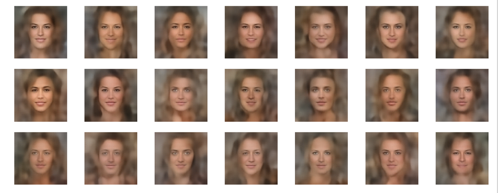
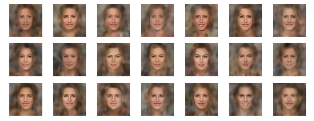
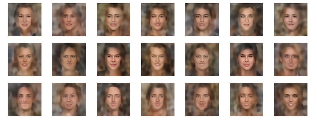
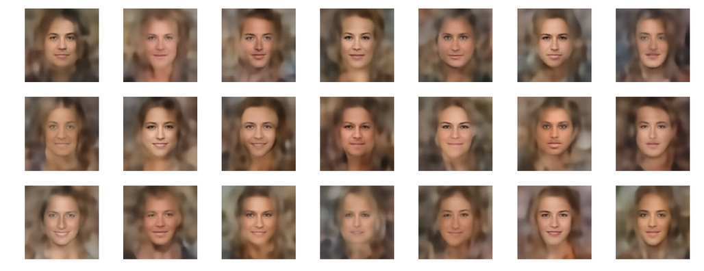
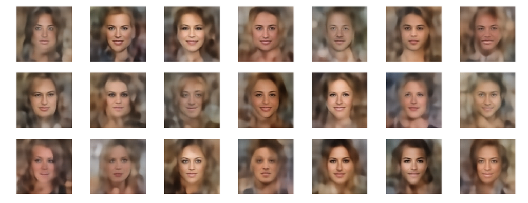
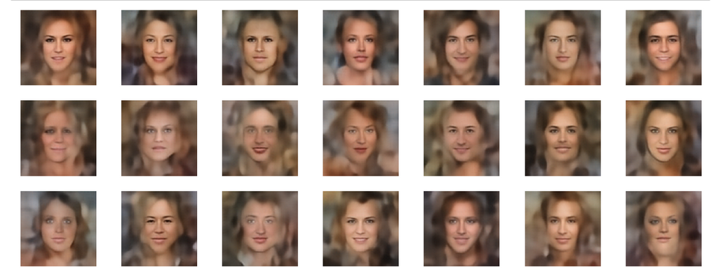
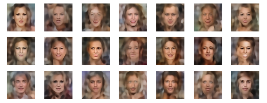
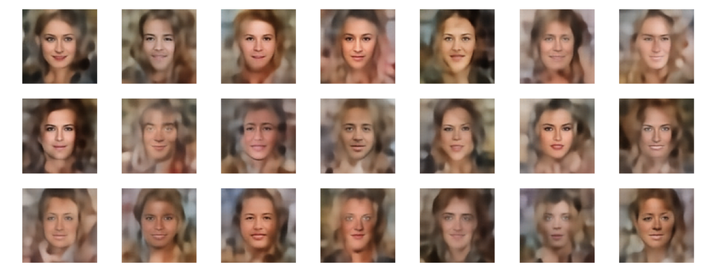
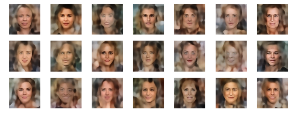
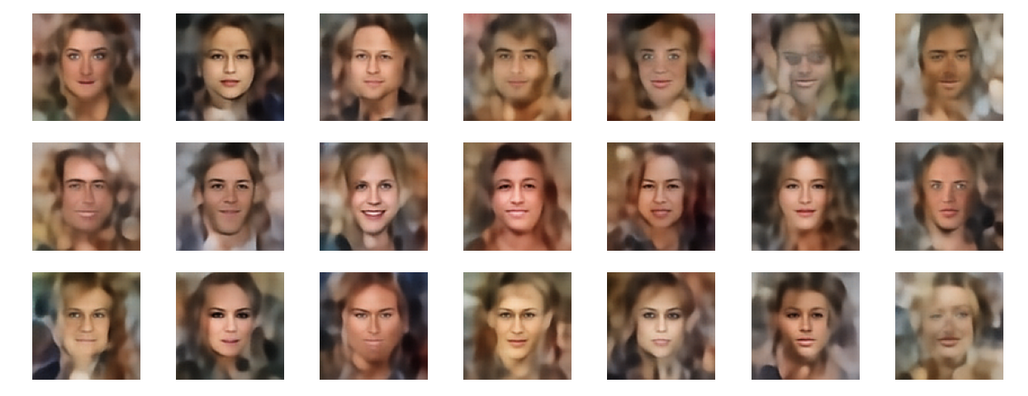
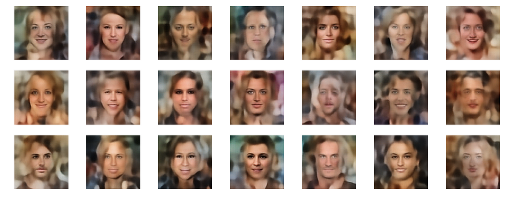
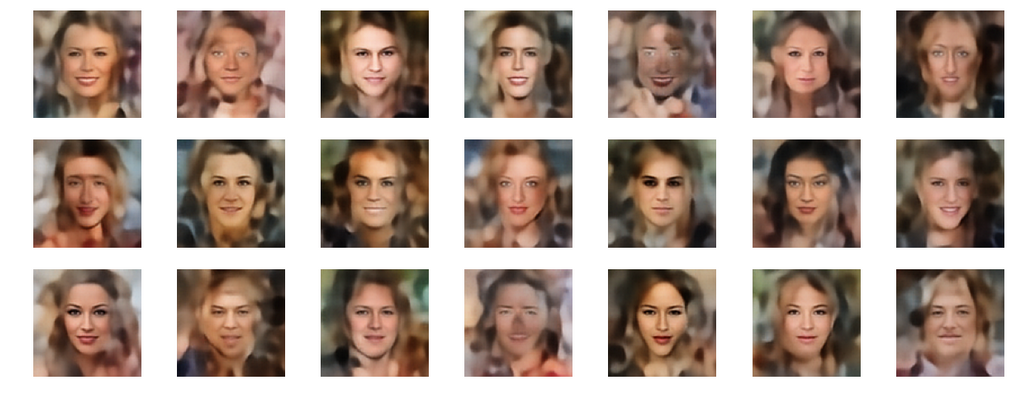
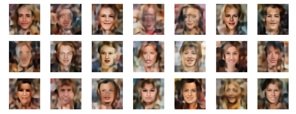
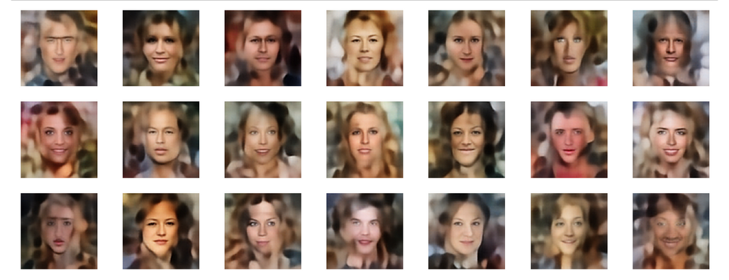
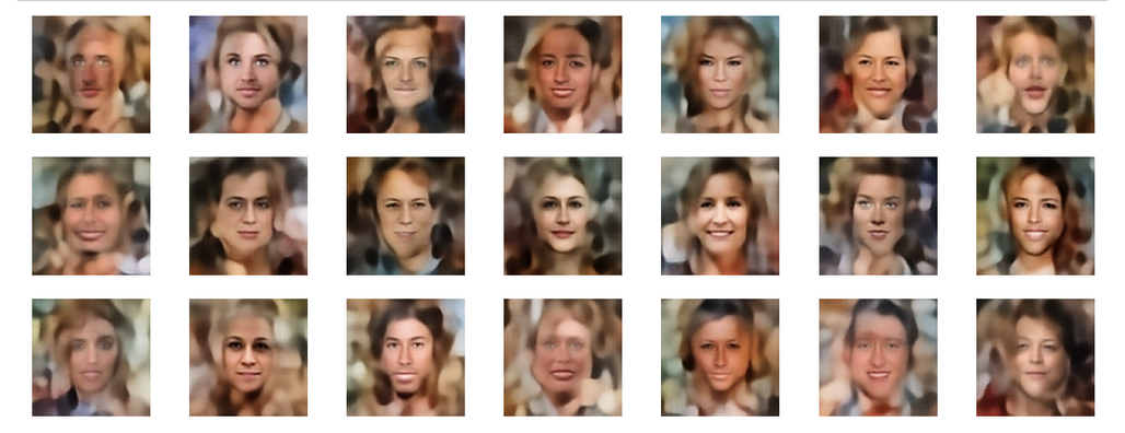
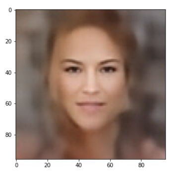
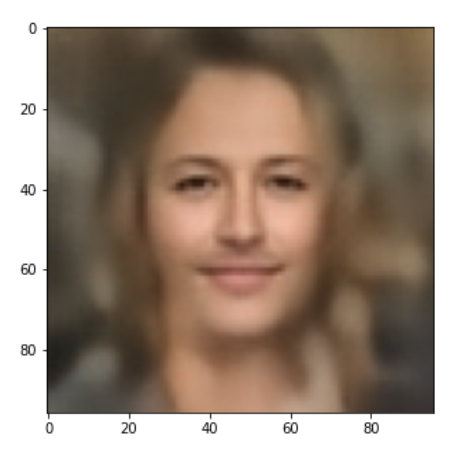
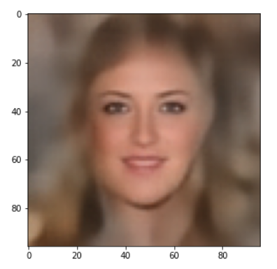
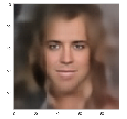
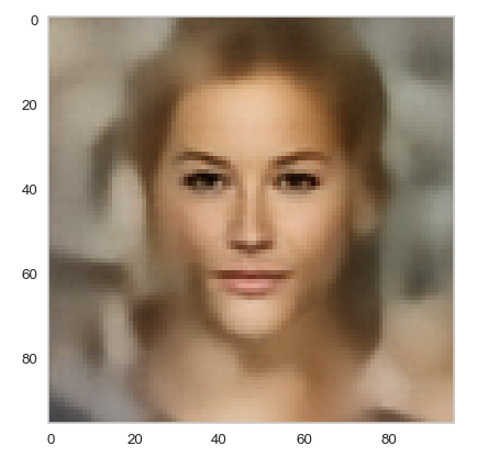
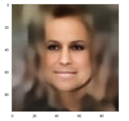
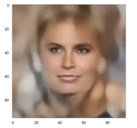
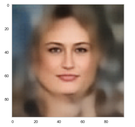
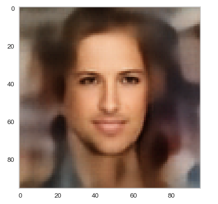
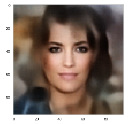
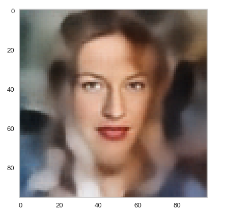
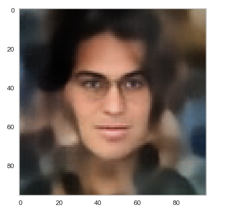
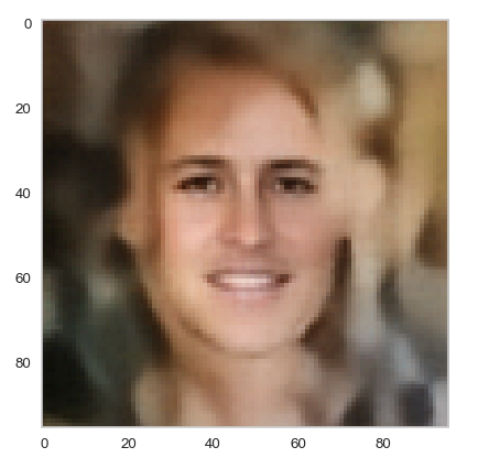
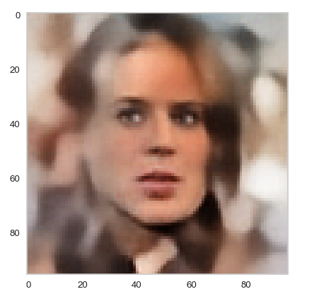
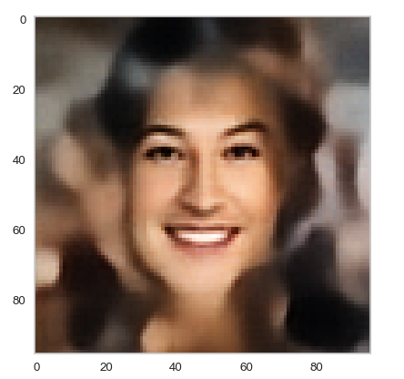
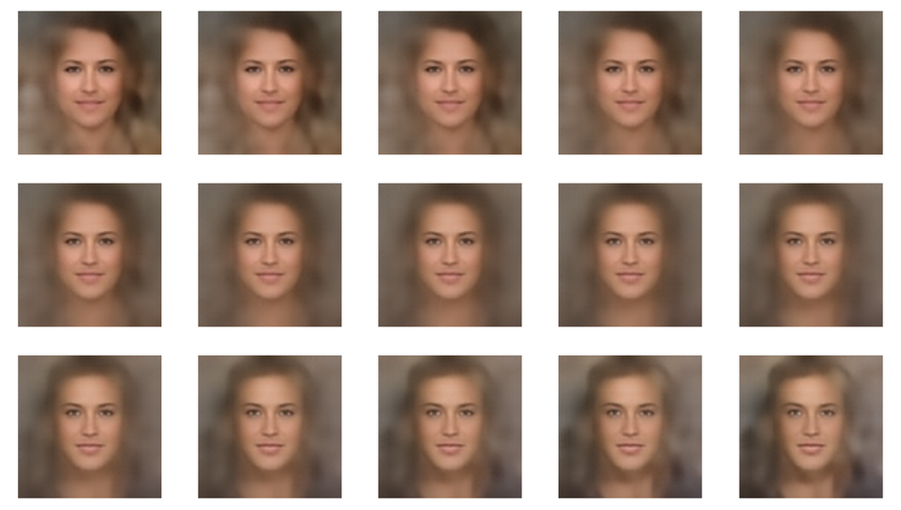
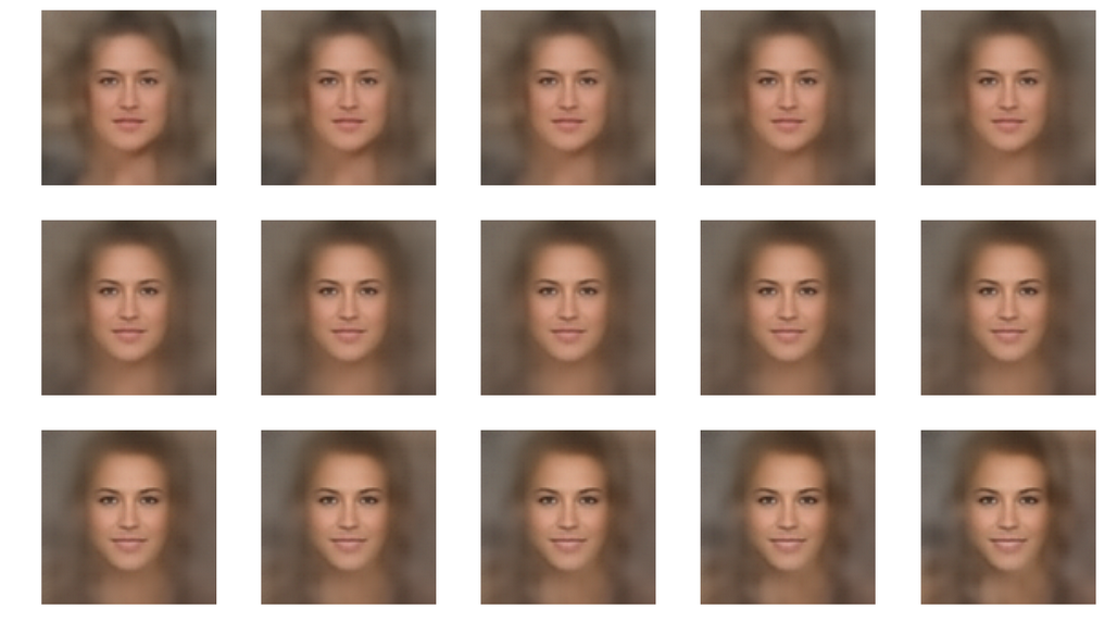
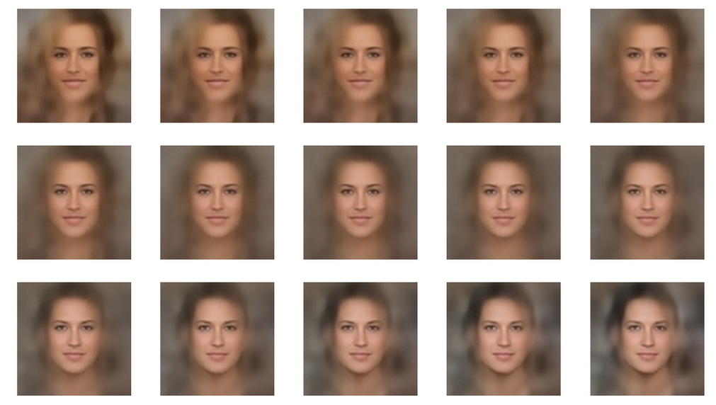
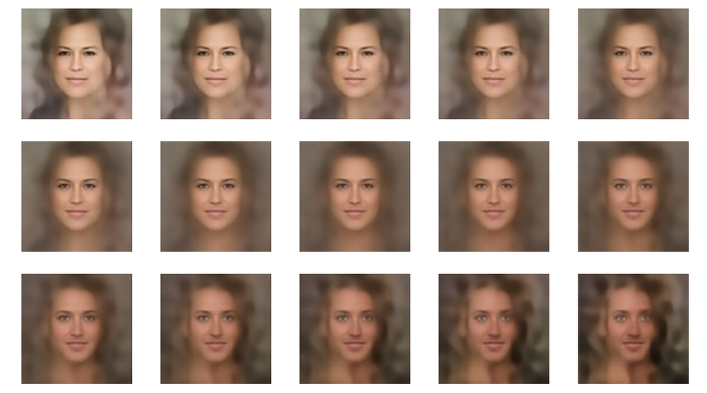
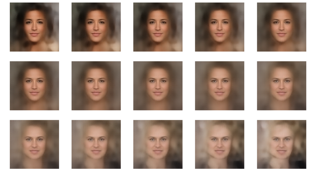
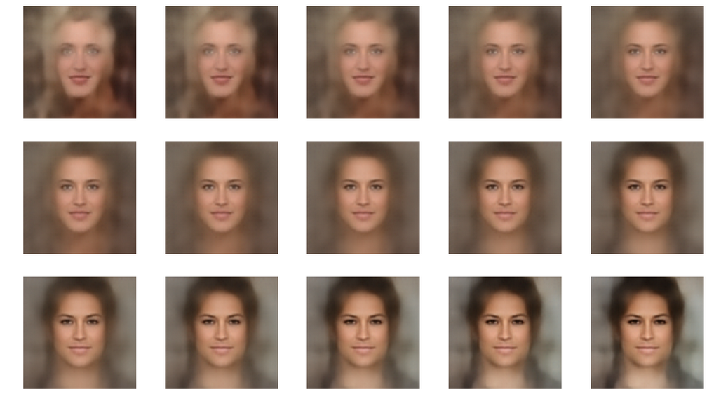
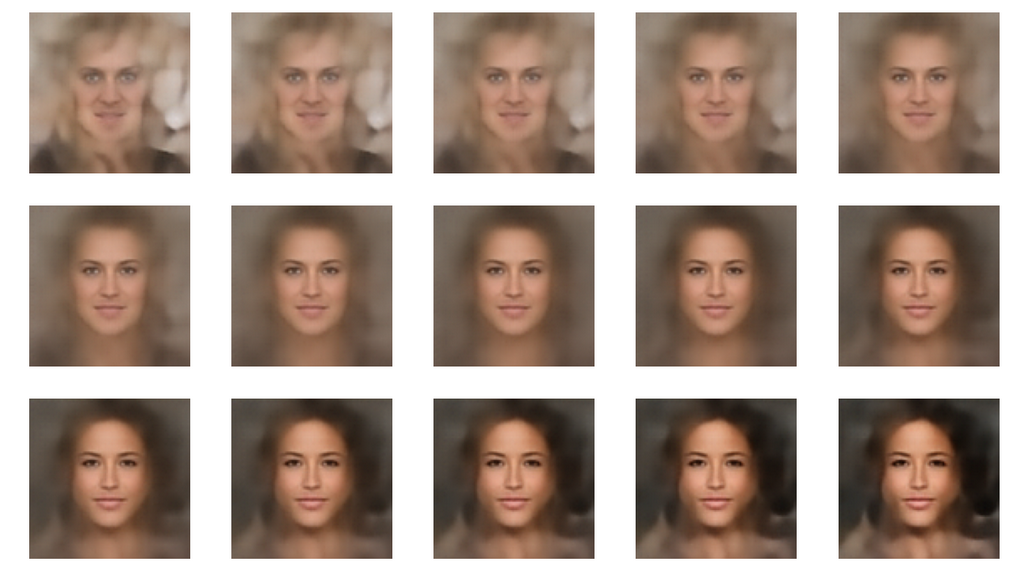
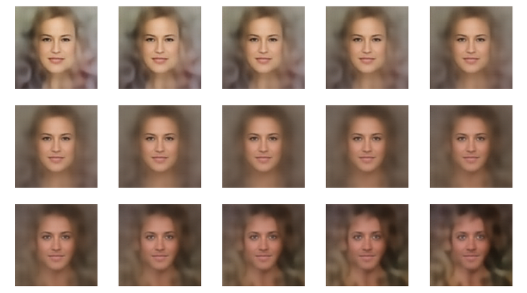
we have trained an AE with images of the CelebA dataset. The Encoder and the Decoder of the AE consist of a series of convolutional layers. Such layers have the ability to extract characteristic patterns out of input (image) data and save related information in their so called feature maps. CelebA images show human heads against varying backgrounds. The AE was obviously able to learn the typical features of human faces, hair-styling, background etc. After a sufficient number of training epochs the AE’s Encoder produces “z-points” (vectors) in the latent space. The latent space is a vector space which has a relatively low number of dimension compared with the number of image pixels. The Decoder of the AE was able to reconstruct images from such z-points which resembled the original closely and with good quality.

We saw, however, that the latent space (or “z-space”) lacks an important property:

The latent space of an Autoencoder does not appear to be densely and uniformly populated by the z-points of the training data.

We saw that his makes the latent space of an Autoencoder almost unusable for creative and generative purposes. The z-points which gave us good reconstructions in the sense of recognizable human faces appeared to be arranged and positioned in a very special way within the latent space. Below I call a CelebA related z-point for which the Decoder produces a reconstruction image with a clearly visible face a “meaningful z-point“.

We could not reconstruct “meaningful” images from randomly chosen z-points in the latent space of an Autoencoder trained on CelebA data. Randomly in the sense of random positions. The Decoder could not re-construct images with recognizable human heads and faces from almost any randomly positioned z-point. We got the impression that many more non-meaningful z-points exist in latent space than meaningful z-points.

We would expect such a behavior if the z-points for our CelebA training samples were arranged in tiny fragments or thin (and curved) filaments inside the multidimensional latent space. Filaments could have the structure of

  • multi-dimensional manifolds with almost no extensions in some dimensions
  • or almost one-dimensional string-like manifolds.

The latter would basically be described by a (wiggled) thin curve in the latent space. Its extensions in other dimensions would be small.

It was therefore reasonable to assume that meaningful z-points are surrounded by areas from which no reasonable interpretable image with a clear human face can be (re-) constructed. Paths from a “meaningful” z-point would only in a very few distinct directions lead to another meaningful point. As it would be the case if you had to follow a path on a thin curved manifold in a multidimensional vector space.

So, we had some good reasons to speculate that meaningful data points in the latent space may be organized in a fragmented way or that they lie within thin and curved filaments. I gave my readers a link to a scientific study which supported this view. But without detailed data or some visual representations the experiments in my last post only provided indirect indications of such a complex z-point distribution. And if there were filaments we got no clue whether these were one- or multidimensional.

Important Addendum, 03/18/2023:

I have to correct this post regarding the basic line of thought: Even if we find that the z-points for CelebA images are arranged in filaments the failure we saw in the first post of this series may not have its direct cause in missing these filaments in latent space by randomly chosen z-points. It could also be that we miss a much larger, coherent region where meaningful points are located. The filaments then would correspond to a correlation of certain features, only, which may not be decisive for the reconstruction of a face. So, the investigation of the existence of filaments is interesting – but the explanation of the AE’s reconstruction failure may require a more thorough analysis. I have done the calculations already, but have not yet found the time to write about them. As soon as the posts are ready I am going to provide a link. See also an added comment at the end of this post.

Do we have a chance to get a more direct evidence about a fragmented or filamental population of the latent space? Yes, I think so. And this is the topic of this post.

However, the analysis is a bit complicated as we have to deal with a multidimensional space. In our case the number of dimensions of the latent space is z_dim = 256. No chance to plot any clusters or filaments directly! However, some other methods will help to reduce the dimensionality of the problem and still get some valid representations of the data point correlations. In the end we will have a very strong evidence for the existence of filaments in the AE’s z-space.

Methods to work with data distributions in many dimensions

Below I will use several methods to investigate the z-point distribution in the multidimensional latent space:

  • An analysis of the variation of the z-point number-density along coordinate axes and vs. radius values.
  • An application of t-SNE projections from the standard multidimensional coordinate system onto a 2-dimensional plane.
  • PCA analysis and subsequent t-SNE projections of the PCA-transformed z-point distribution and its most important PCA components down to a 2-dim plane. Note that such an approach corresponds to a sequence of projections:
    1) Linear projections onto PCA rotated coordinates.
    2) A non-linear SNE-projection which scales and represents data point correlations on different scales on a 2-dim plane.
  • A direct view on the data distribution projected onto flat planes formed by two selected coordinate axes in the PCA-coordinate system. This will directly reveal whether the data (despite projection effects exhibit filaments and voids on some (small ?) scales.
  • A direct view on the data distribution projected onto a flat plane formed by two coordinate axes of the original latent space.

The results of all methods combined strongly support the claim that the latent space is neither populated densely nor uniformly on (small) scales. Instead data points are distributed along certain filamental structures around voids.

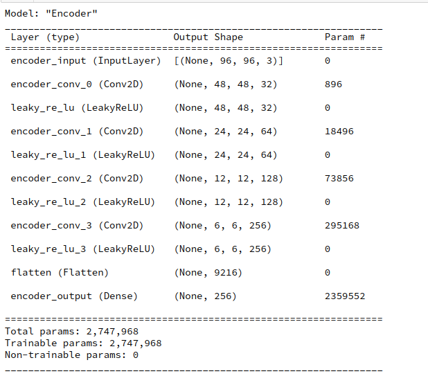
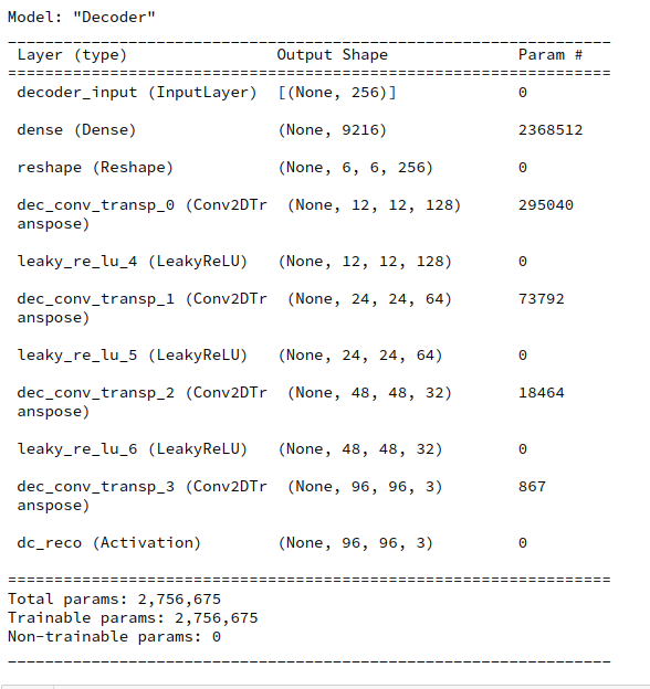
Layer structure of the Autoencoder

Below you find the layer structure of the AE’s Encoder. It got four Conv2D layers. The Decoder has a corresponding reverse structure consisting of Conv2DTranspose layers. The full AE model was constructed with Keras. It was trained on CelebA for 24 epochs with a small step size. The original CelebA images were reduced to a size of 96×96 pixels.

Encoder

Decoder

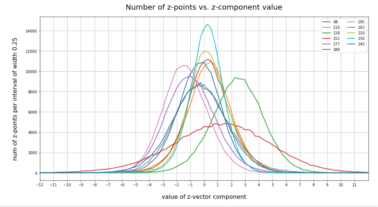
Number density of z-points vs. coordinate values

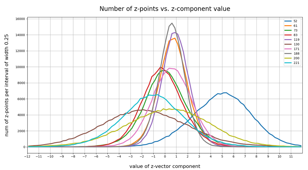
Each z-point can be described by a vector, whose components are given by projections onto the 256 coordinate axes. We assume orthogonal axes. Let us first look at the variation of the z-point number density vs. reasonable values for each of the 256 vector-components.

Below I have plotted the number density of z-points vs. coordinate values along all 256 coordinate axes. Each curve shows the variation along one of the 256 axes. The data sampling was done on intervals with a width of 0.25:

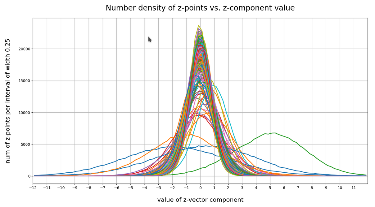
Most curves look like typical Gaussians with a peak at the coordinate value 0.0 with a half-width of around 2.

You see, however, that there are some coordinates which dominate the spatial distribution in the latent vector-space. For the following components the number density distribution is relatively broad and peaks at a center different from the origin of the z-space. To pick a few of these coordinate axes:

 52, center:  5.0,  width: 8
 61; center;  1.0,  width: 3 
 73; center:  0.0,  width: 5.5  
 83; center: -0.5,  width: 5
 94; center:  0.0,  width: 4
116; center:  0.0,  width: 4
119; center:  1.0,  width: 3
130; center: -2.0,  width: 9
171; center:  0.7,  width: 5
188; center:  0.75, width: 2.75
200; center:  0.5,  width: 11
221; center: -1.0,  width: 8

The first number is just an index of the vector component and the related coordinate axis. The next plot shows the number density along some these specific coordinate axes:

What have we learned?
For most coordinate axes of the latent space the number density of the z-points peaks at 0.0. We see an approximate Gaussian form of the number density distribution. There are around 5 coordinate directions where the distribution has a peak significantly off the origin (52, 130, 171, 200, 221). Along the corresponding axes the distribution of z-points obviously has an elongated form.

If there were only one such special vector component then we would speak of an elongated, ellipsoidal and almost cigar like distribution with the thickest area at some position along the specific coordinate axis. For a combination of more axes with elongated distributions, each with with a center off the origin, we get instead diagonally oriented multidimensional and elongated shapes.

These findings show again that large regions of the latent space of an AE remain empty. To get an idea just imagine a three dimensional space with all data in x-direction culminating at a coordinate value of 5 with a half-width of lets say 8. In the other directions y and z we have our Gaussian distributions with a total half-width of 1 around the mean value 0. What do we get? A cigar like shape confined around the x-axis and stretching from -3 < x < 13. And the rest of the space: More or less empty. We have obviously found something similar at different angular directions of our multidimensional latent space. As the number of special coordinate directions is limited these findings tell us that a PCA analysis could be helpful. But let us first have a look at the variation of number density with the radius value of the z-points.

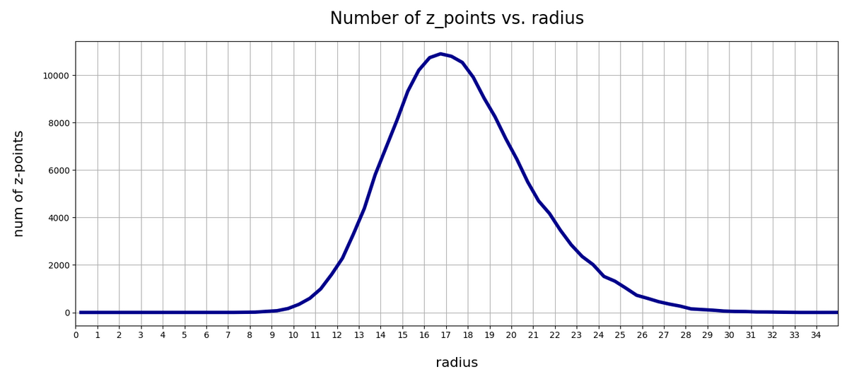
Number density of z-points vs. radius

We define a radius via an Euclidean L2 norm for our 256-dimensional latent space. Afterward we can reduce the visualization of the z-point distribution to a one dimensional problem. We can just plot the variation of the number density of z-points vs. the radius of the z-points.

In the first plot below the sampling of data was done on intervals of 0.5 .

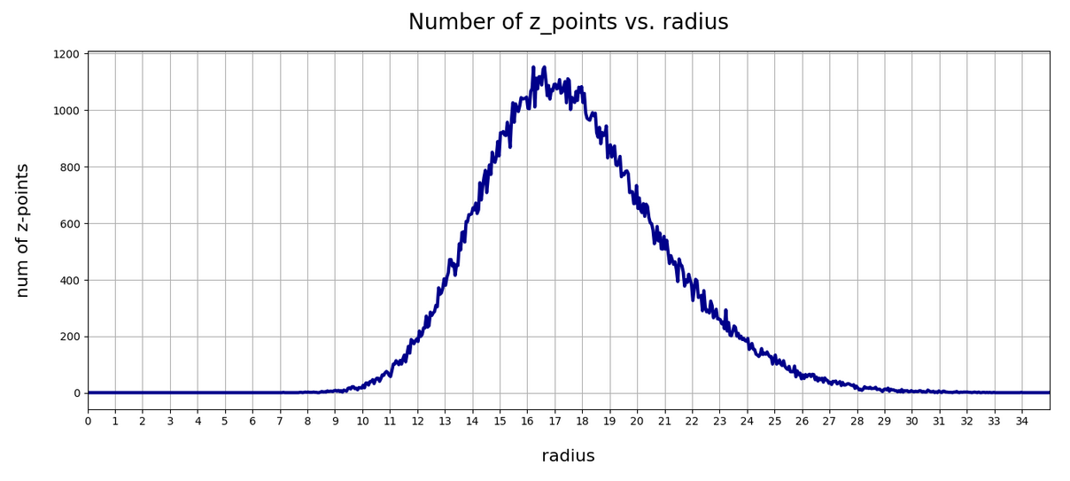
The curve does not remain that smooth on smaller sampling intervals. See e.g. for intervals of width 0.05

Still, we find a pronounced peak at a radius of R=16.5. But do not get misguided: 16 appears to be a big value. But this is mainly due to the high number of dimensions!

How does the peak in the close vicinity of R=16 fit to the above number density data along the coordinate axes? Answer: Very well. If you assume a z-point vector with an average value of 1 per coordinate direction we actually get a radius of exactly R=16!

But what about Gaussian distributions along the coordinate axes? Then we have to look at resulting expectation values. Let us assume that we fill a vector of dimension 256 with numbers for each component picked statistically from a normal distribution with a width of 1. And let us repeat this process many times. Then what will the expectation value for each component be?

A coordinate value contributes with its square to the radius. The math, therefore, requires an evaluation of the integral integral[(x**2)*gaussian(x)] per coordinate. This integral gives us an expectation value for the contribution of each coordinate to the total vector length (on average). The integral indeed has a resulting value of 1.0. From this it follows that the expectation value for the distance according to an Euclidean L2-metric would be avg_radius = sqrt(256) = 16. Nice, isn’t it?

However, due to the fact that not all Gaussians along the coordinate axes peak at zero, we get, of course, some deviations and the flank of the number distribution on the side of larger radius values becomes relatively broad.

What do we learn from this? Regions very close to the origin of the z-space are not densely populated. And above a radius value of 32, we do not find z-points either.

t-SNE correlation analysis and projections onto a 2-dimensional plane

To get an impression of possible clustering effects in the latent space let us apply a t-SNE analysis. A non-standard parameter set for the sklearn-variant of t-SNE was chosen for the first analysis

tsne2 = TSNE(n_components, early_exaggeration=16, perplexity=10, n_iter=1000) 

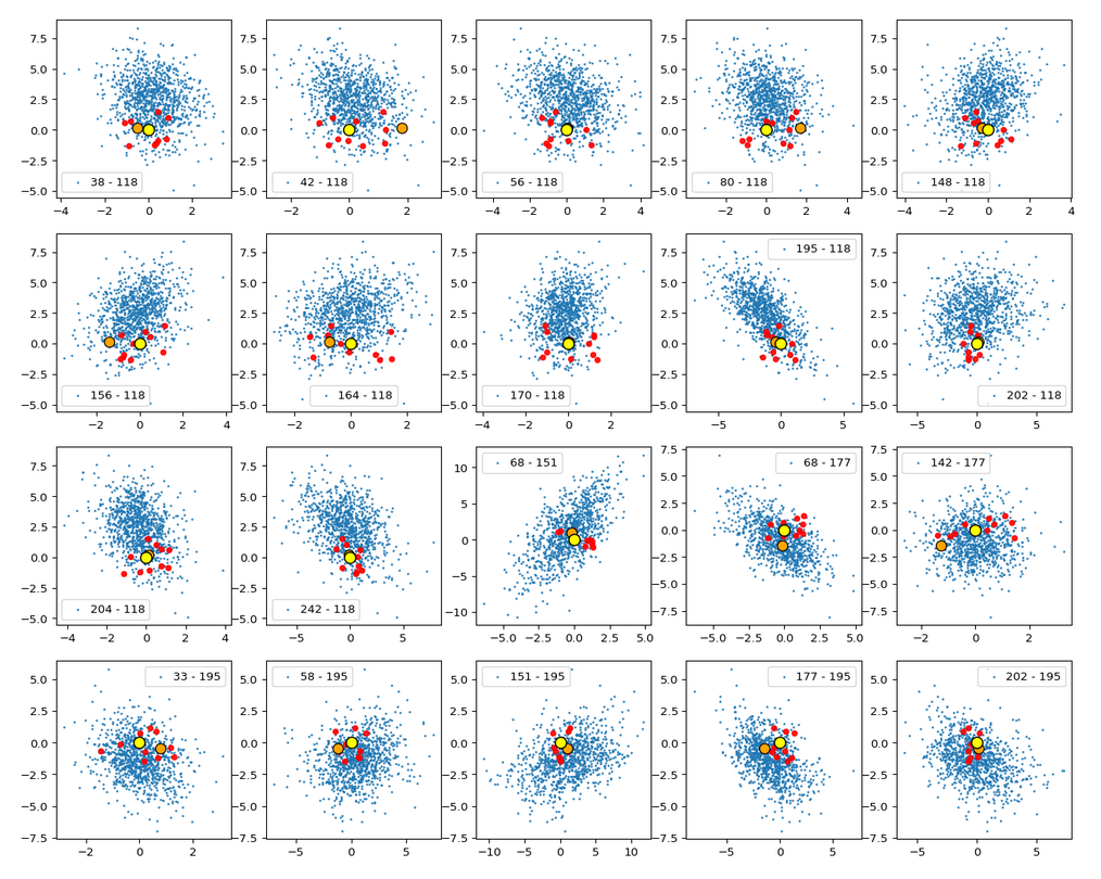
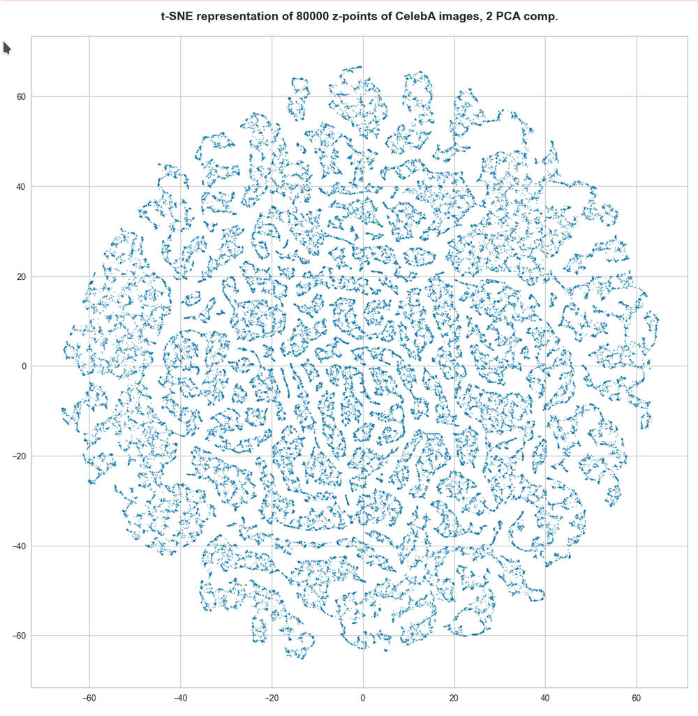
The first plot shows the result for 20,000 randomly selected z-points corresponding to CelebA images

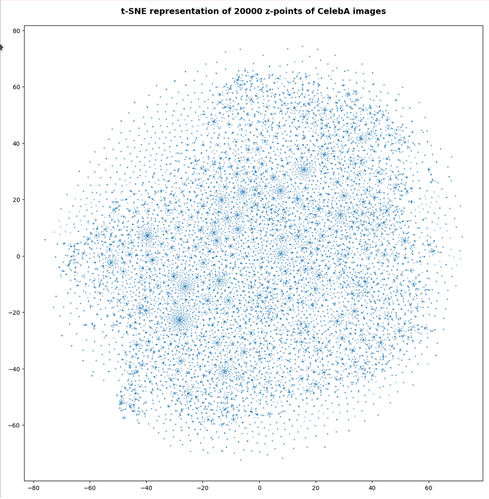
Also this plot indicates that the latent space is not populated with uniform density in all regions. Instead we see some fragmentation and clustering. But note that this might happened on different length scales. t-SNE arranges its projections such that correlations on different scales get clearly indicated. So the distances in this plot must not be confused with the real spatial distances in the original latent space. The axes of the t-SNE plot do not reflect any axes of the latent space and the plotted distribution is not the real data point distribution after a linear and orthogonal projection onto a plane. t-SNE works non-linearly.

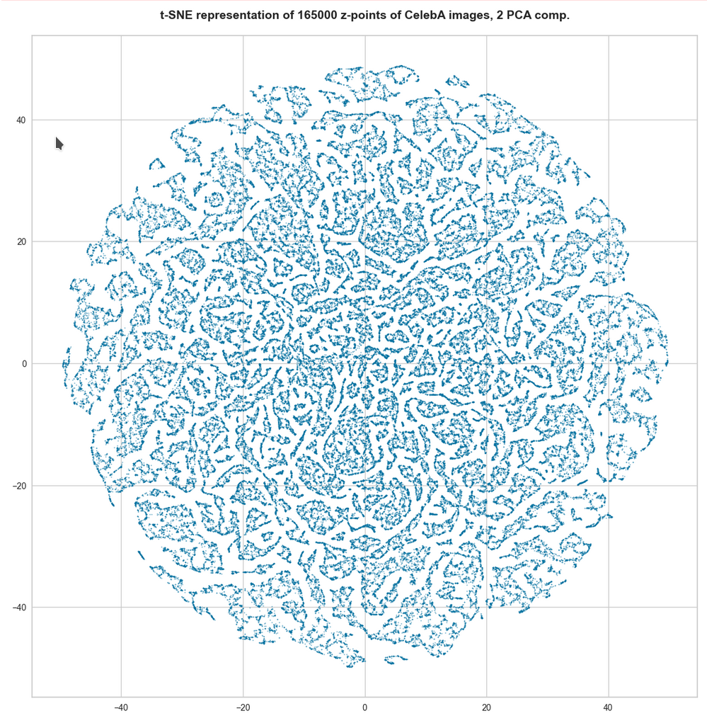
However, the impression of clustering remains for a growing numbers of z-points. In contrast to the first plot the next plots for 80,000 and 165,000 z-points were calculated with standard t-SNE parameters.

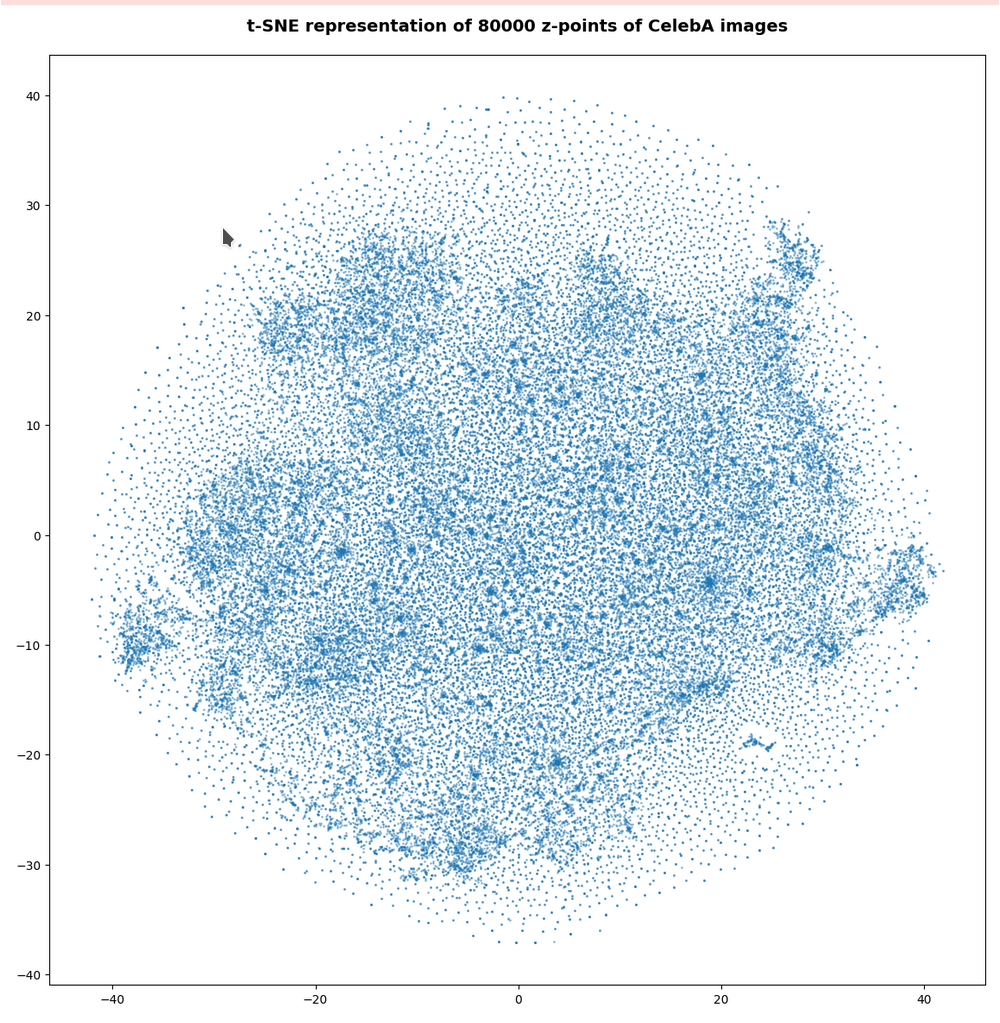
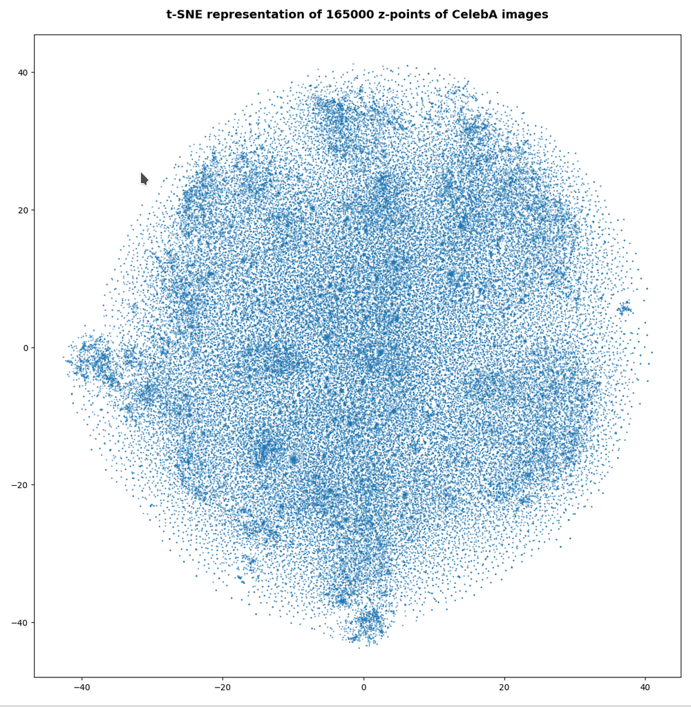
We still see gaps everywhere between locally dense centers. At the center the size of the plotted points leads to overlapping. If one could zoom into some of the centers then gaps would again appear on smaller scales (see more plots below).

PCA analysis and t-SNE-plots of the z-point distribution in the (rotated) PCA coordinate system

The z-point distribution can be analyzed by a PCA algorithm. There is one dominant component and the importance smooths out to an almost constant value after the first 10 components.

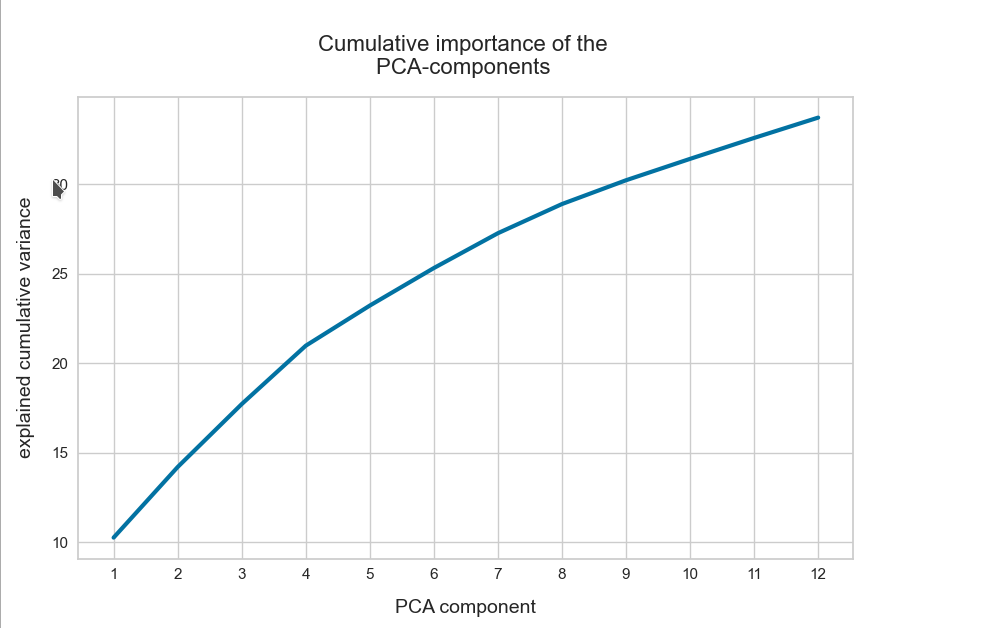
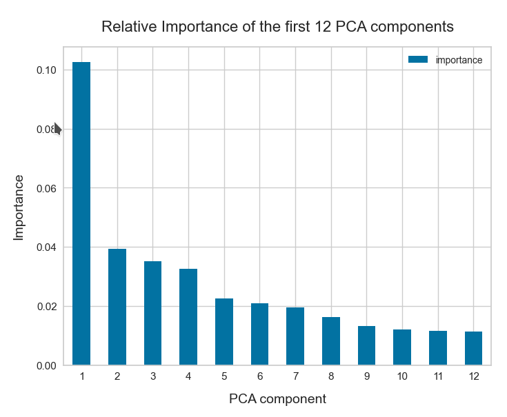
This is consistent with the above findings. Most of the coordinates show rather similar Gaussian distributions and thus contribute in almost the same manner.

The PCA-analysis transforms our data to a rotated coordinate system with a its origin at a position such that the transformed z-point distribution gets centered around this new origin. The orthogonal axes of the new PCA-coordinates system show into the direction of the main components.

When the projection of all points onto planes formed by two selected PCA axes do not show a uniform distribution but a fragmented one, then we can safely assume that there really is some fragmentation going on.

t-SNE after PCA

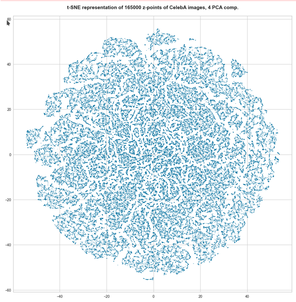
Below you see t-SNE-plots for a growing number of leading PCA components up to 4. The filamental structure gets a bit smeared out, but it does not really disappear. Especially the elongated empty regions (voids) remain clearly visible.

t-SNE after PCA for the first 2 main components – 80,000 randomly selected z-points

t-SNE after PCA for the first 2 main components – 165,000 randomly selected z-points

t-SNE after PCA for the first 4 main PCA components – 165,000 randomly selected z-points

For 10 components t-SNE gets a presentation problem and the plots get closer to what we saw when we directly operated on the latent space.

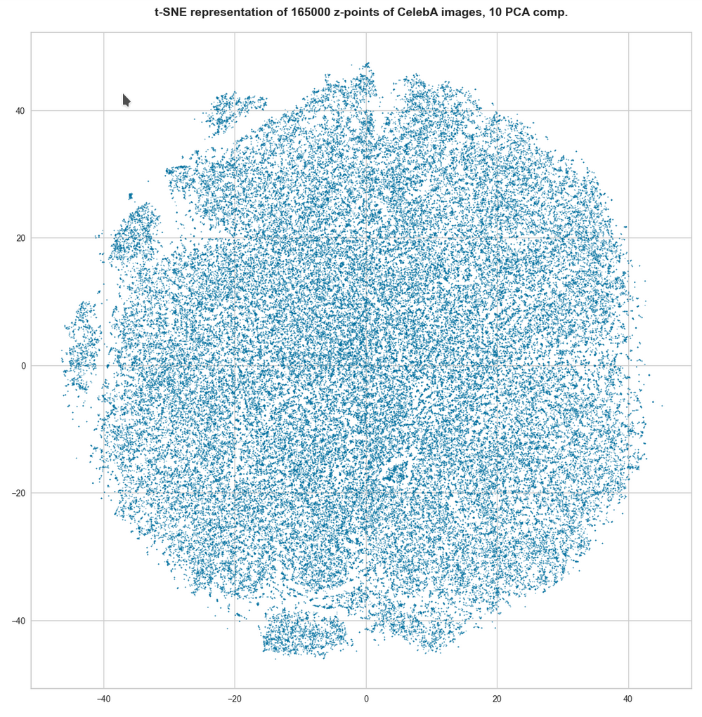
But still the 10-dim space does not appear to be uniformly populated. Despite an expected smear out effect due to the non-linear projection the empty ares seem to be at least as many and as extended as the populated areas.

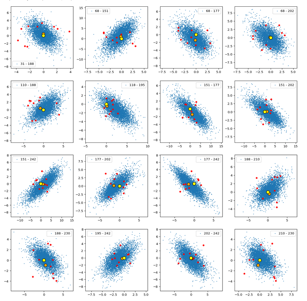
Direct view on the z-point distribution after PCA in the rotated and centered PCA coordinate system

t-SNE blows correlations up to make them clearly visible. Therefore, we should also answer the following question:

On what scales does the fragmentation really happen ?

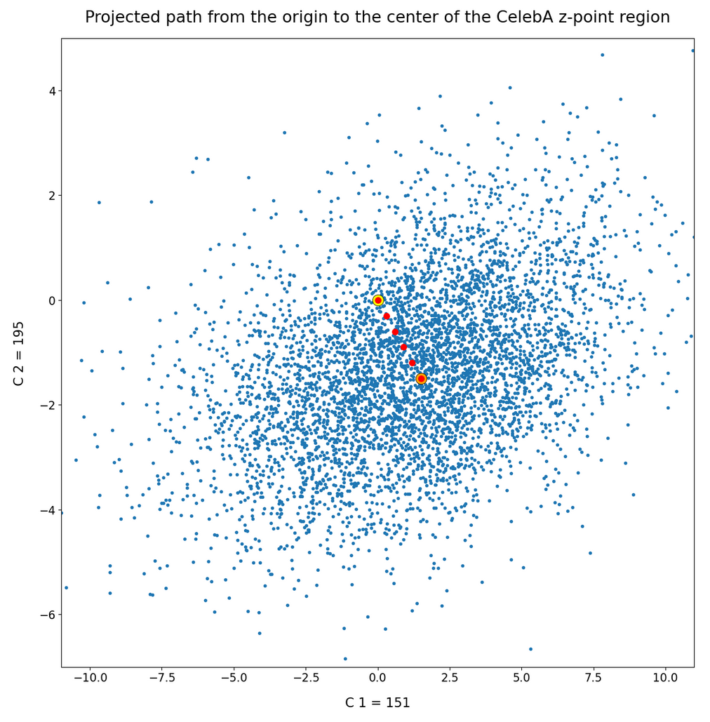
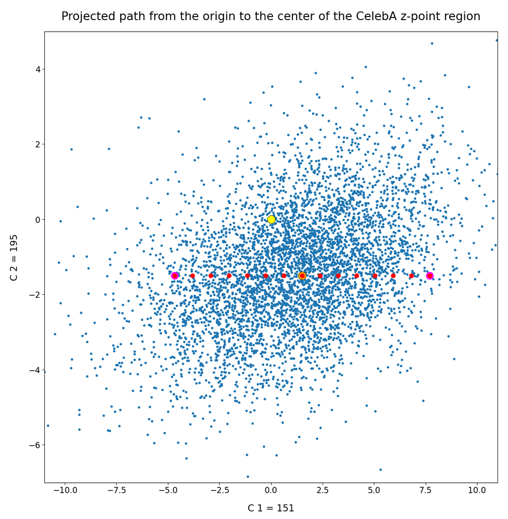
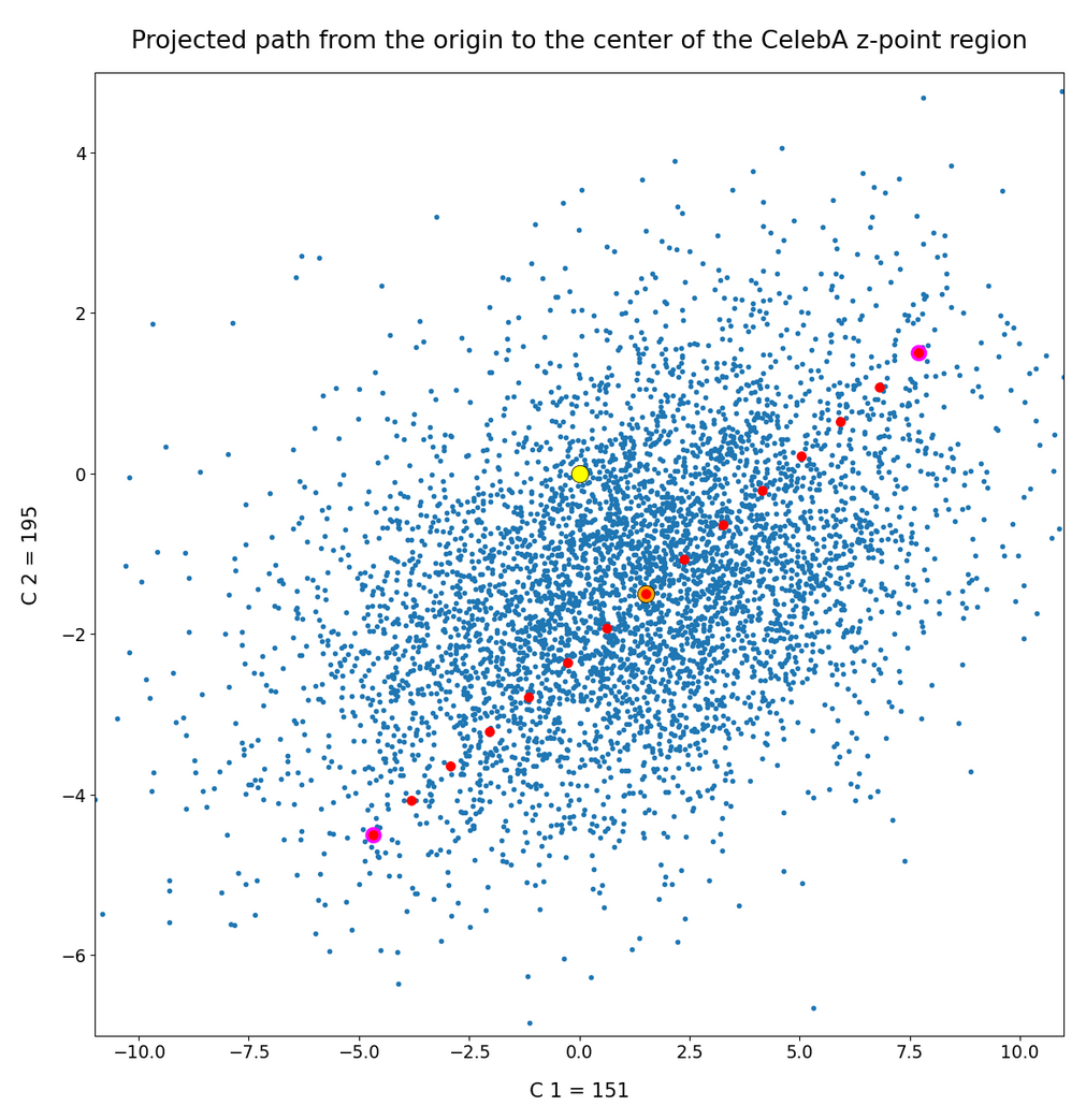
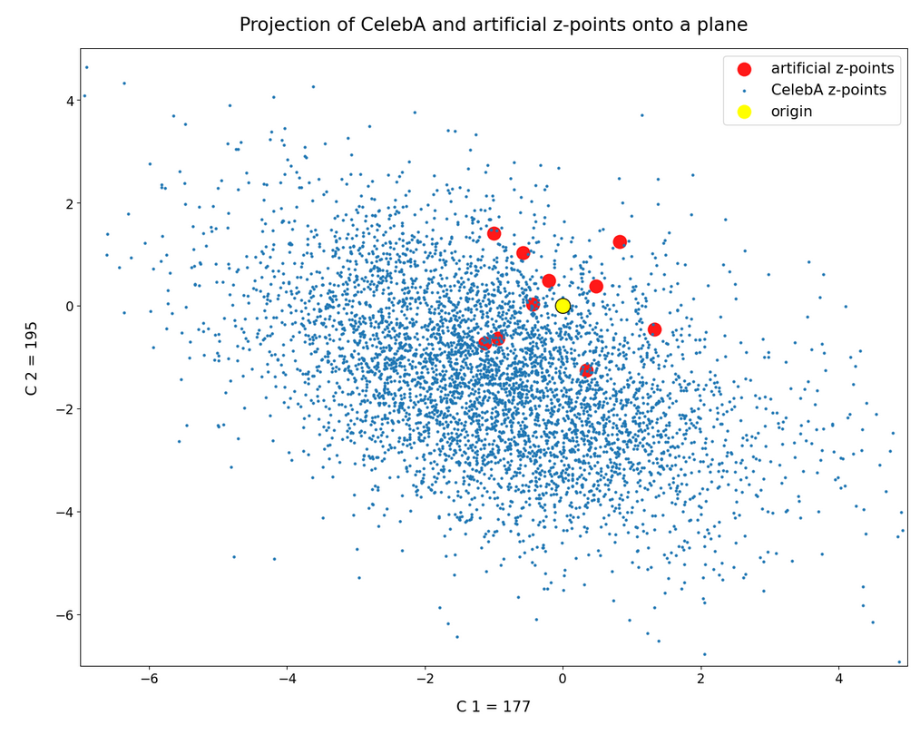
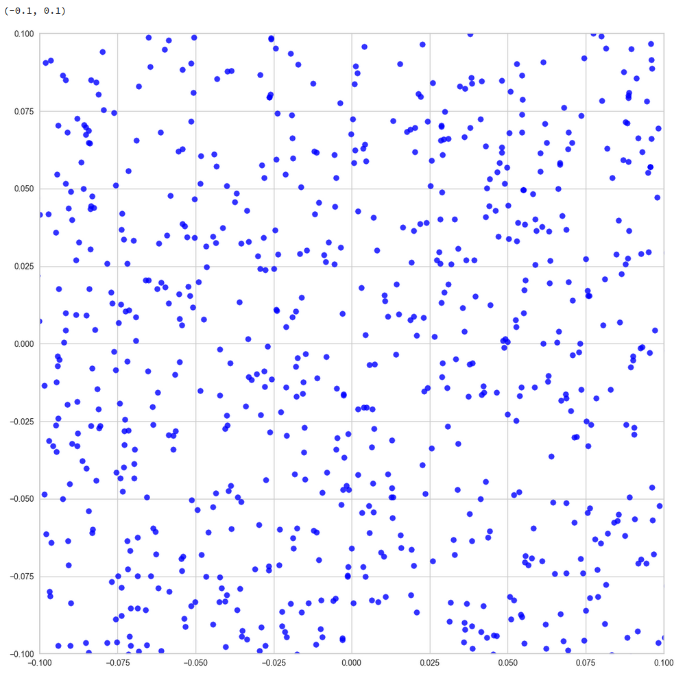
For this purpose we can make a scatter plot of the projection of the z-points onto a plane formed by the leading two primary component axes. Let us start with an overview and relatively large limiting values along the two (PCA) axes:

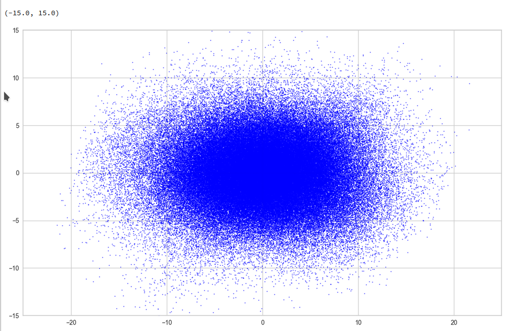
Yeah, a PCA transformation obviously has centered the distribution. But now the latent space appears to be filled densely and uniformly around the new origin. Why?

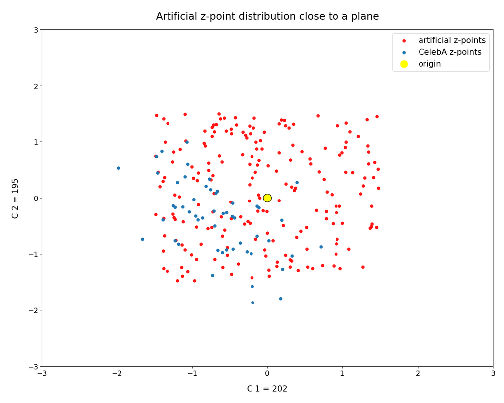
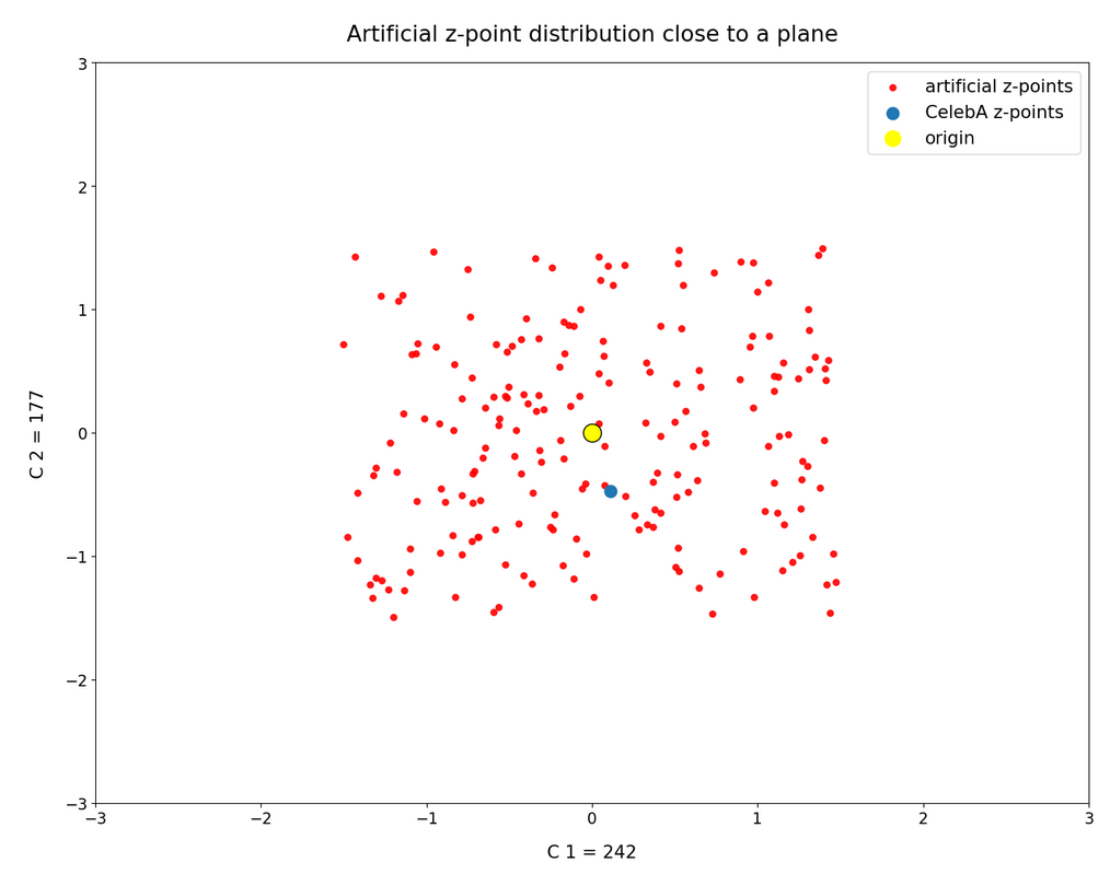
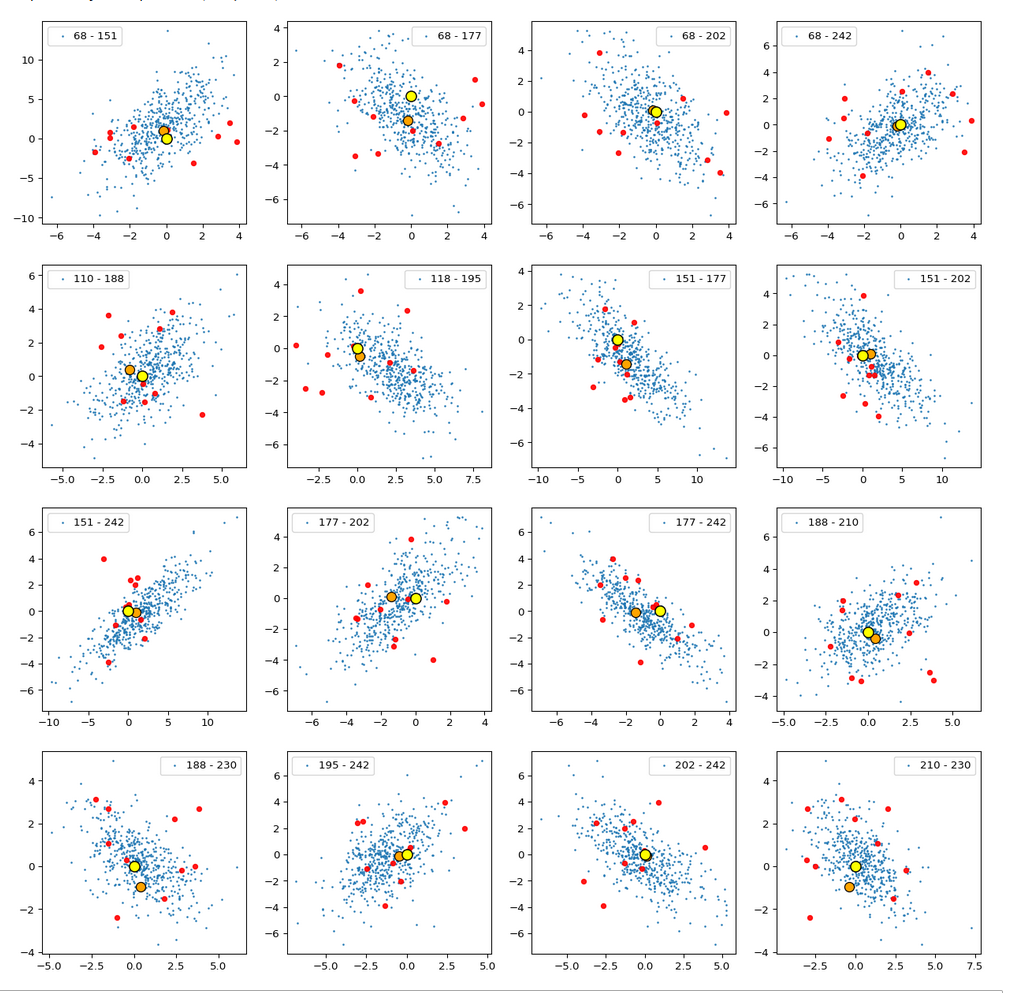
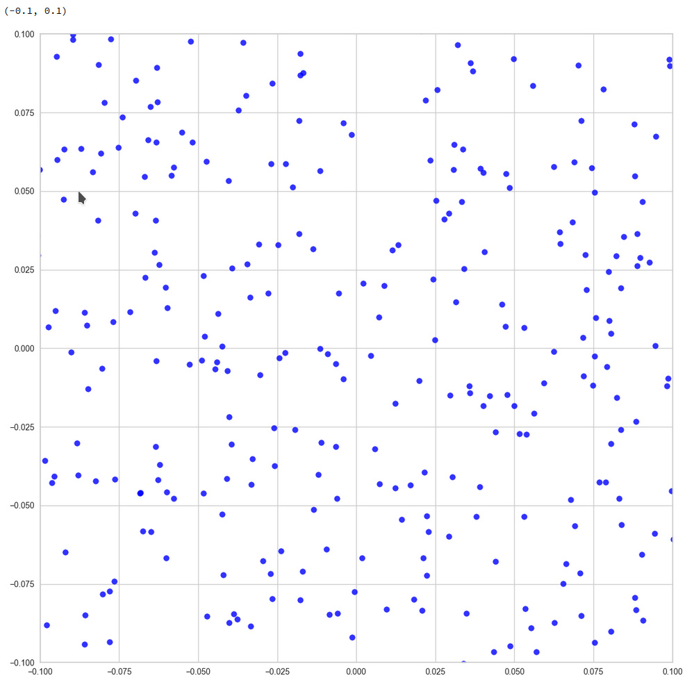
Well, this is only a matter of the visualized length scales. Let us zoom in to a square of side-length 5 at the center:

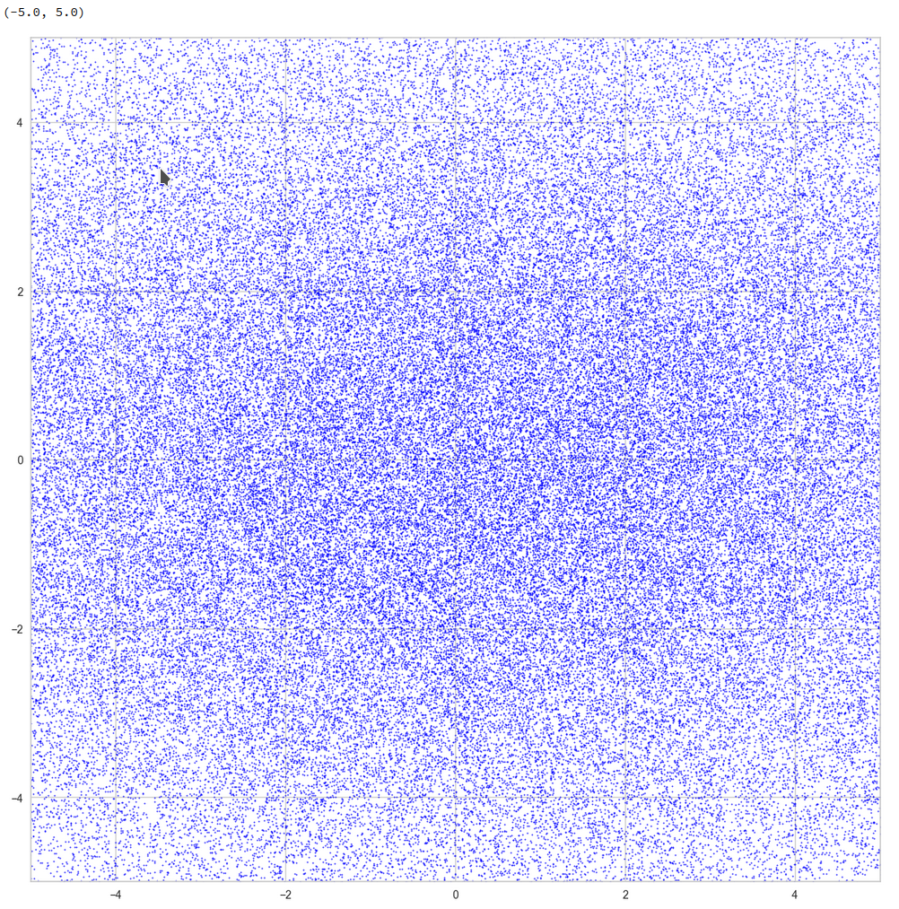
Well, not so densely populated as we thought.

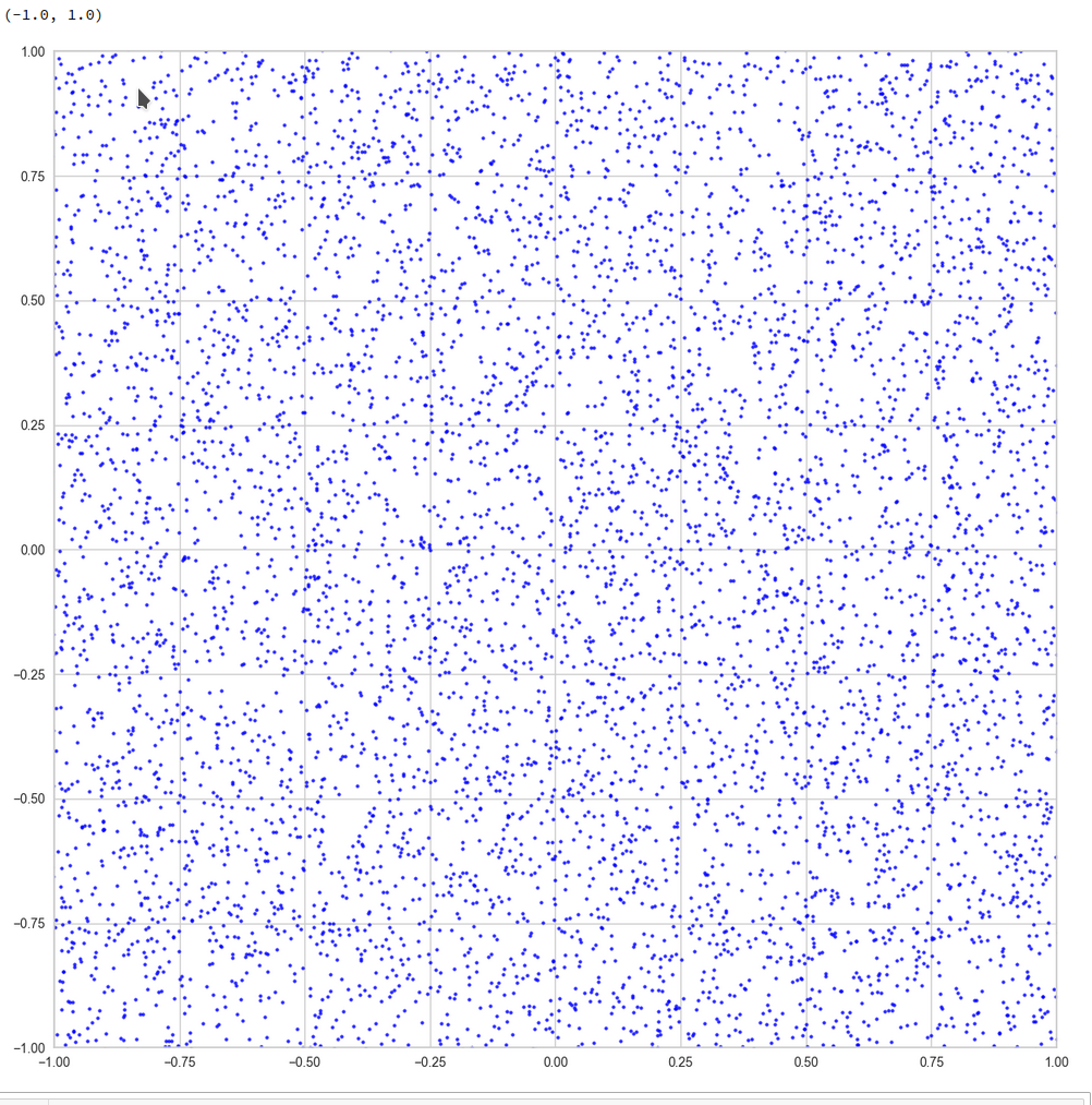
And yet a further zoom to smaller length scales:

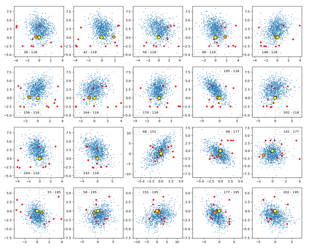
And eventually a really small square around the origin of the PCA coordinate system:

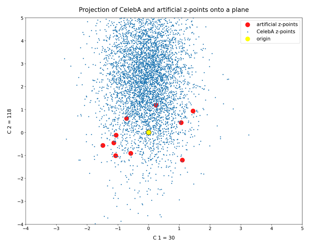
z-point distribution at the center of a two-dim plane formed by the coordinate axes of the first 2 primary components
The chosen qsquare has its corners at (-0.25, -0.25), (-0.25, 0.25), (0.25, -0.25), (0.25, 0.25).

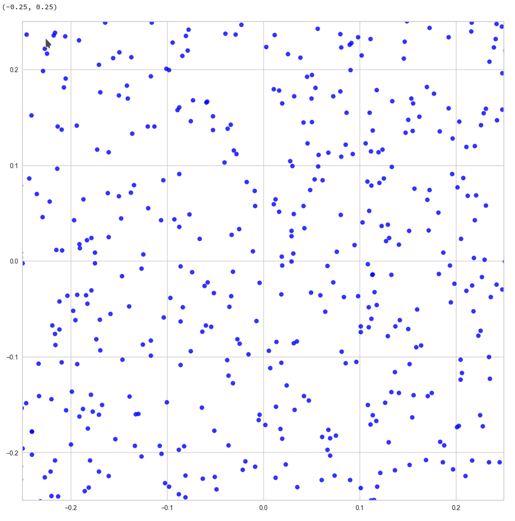
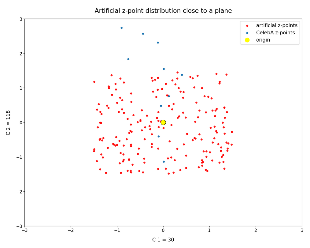
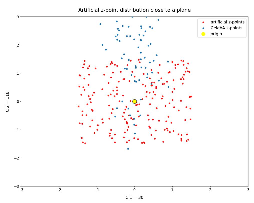
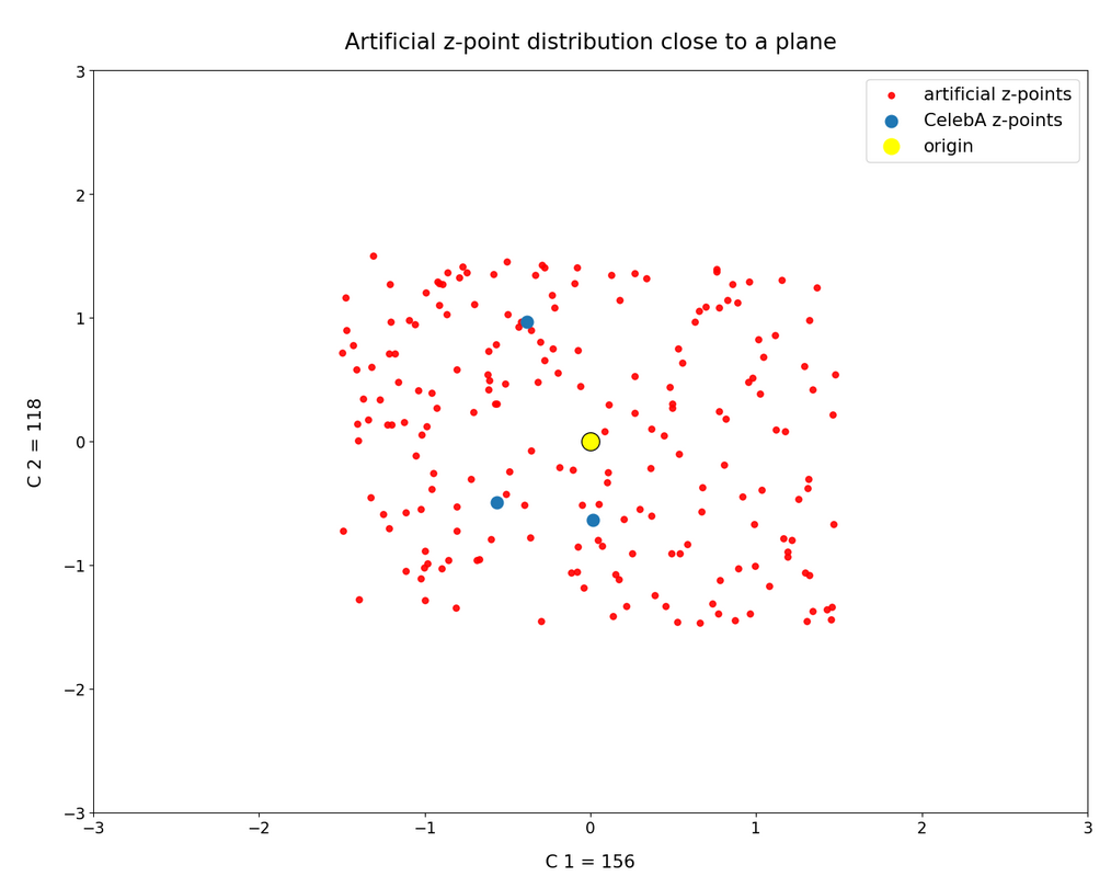
Obviously, not a dense and neither a uniform distribution! After a PCA transformation we see the still see how thinly the latent space is populated and that the “meaningful” z-points from the CelebA data lie along curved and narrow lines or curves with some point-like intersections. Between such lines we see extended voids.

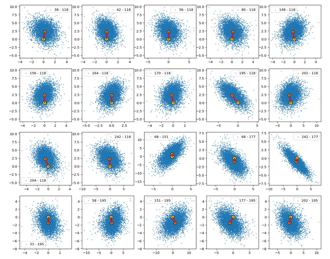
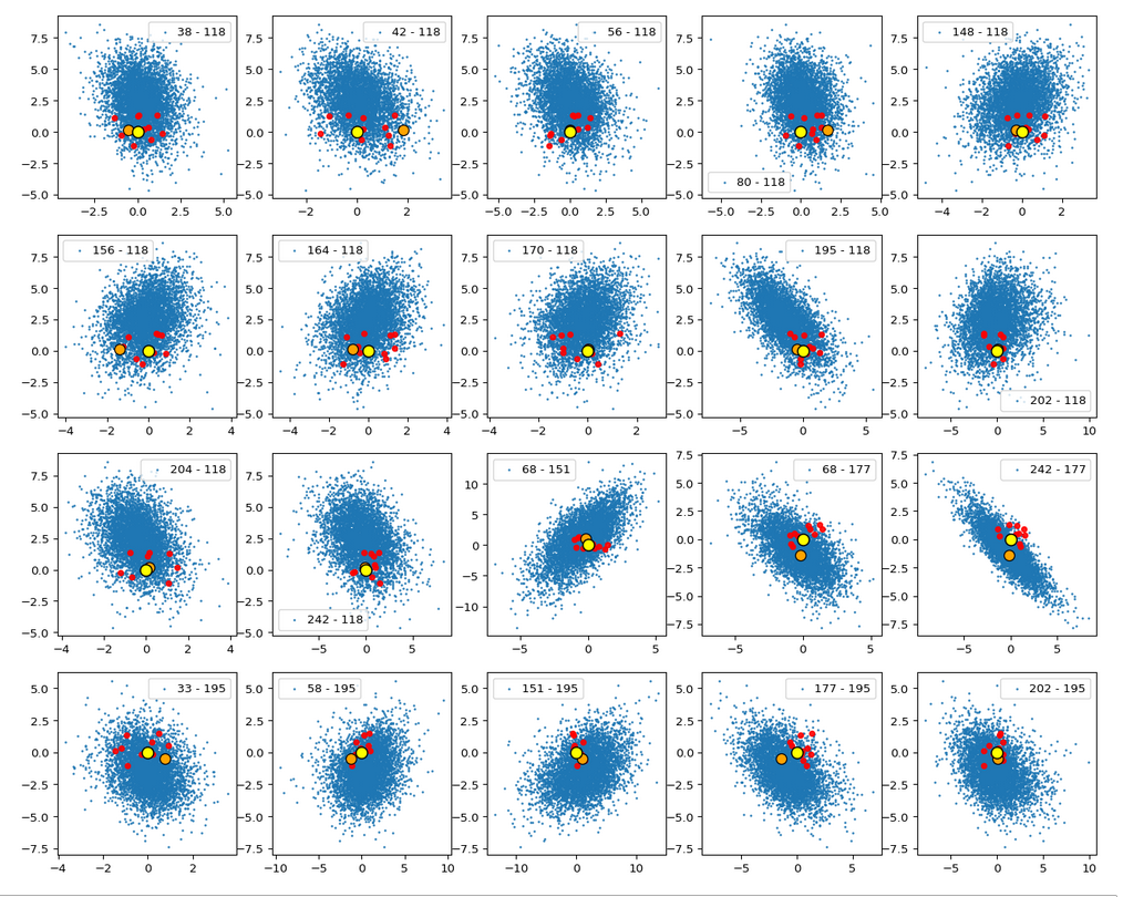
Let us see what happens when we look at the 2-dim pane defined by the first and the 18th axes of the PCA coordinate system:

Or the distribution resulting for the plane formed by the 8th and the 35th PCA axis:

We could look at other flat planes, but we do not get rid of he line like structures around void like areas. This is really a strong indication of filamental structures.

Interpretation of the line patterns:
The interesting thing is that we get lines for z-point projections onto multiple planes. What does this tell us about the structure of the filaments? In principle we have the two possibilities already named above: 1) Thin multidimensional manifolds or 2) thin and basically one-dimensional manifolds. If you think a bit about it, you will see that projections of multidimensional manifolds would not give us lines or curves on all projection planes. However curved string- or tube-like manifolds do appear as lines or line segments after a projection onto almost all flat planes. The prerequisite is that the extension of the string in other directions than its main one must really be small. The filament has to have a small diameter in all but one directions.

So, if the filaments really are one-dimensional string-like objects: Should we not see something similar in the original z-space? Let us for example look at the plane formed by axis 52 and axis 221 in the original z-space (without PCA transformation). You remember that these were axes where the distribution got elongated and had centers at -2 and 5, respectively. And indeed:

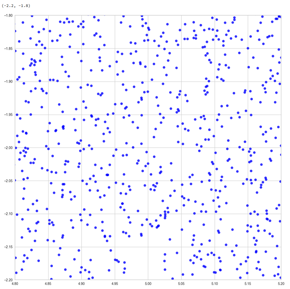
Again we see lines and voids. And this strengthens our idea about filaments as more or less one-dimensional manifolds.

The “meaningful” z-points for our CelebA data obviously get positioned on long, very thin and basically one-dimensional filaments which surround voids. And the voids are relatively large regarding their area/volume. (Reminds me of the galaxy distribution in simulations of the development of the early universe, by the way.)

Therefore: Whenever you chose a randomly positioned z-point the chance that you end up in an unpopulated region of the z-space or in a void and not on a filament is extremely big.

Conclusion

We have used a whole set of methods to analyze the z-point distribution of an AE trained on CelebA images. We found the the z-point distribution is dominated by the number density variation along a few coordinate axes. Elongated shapes in certain directions of the latent space are very plausible on larger scales.

We found that the number density distributions along most of the coordinate axes have a thin Gaussian form with a peak at the origin and a half-with of 1. We have no real explanation for this finding. But it may be related to the fact the some dominant features of human faces show Gaussian distributions around a mean value. With Gaussians given we could however explain why the number density vs. radius showed a peak close to R=16.

A PCA analysis finds primary directions in the multidimensional space and transforms the z-point distribution into a corresponding one for orthogonal primary components axes. For logical reason we can safely assume that the corresponding projections of the z-point distribution on the new axes would still reveal existing thin filamental structures. Actually, we found lines surrounding voids independently onto which flat plane we projected the data. This finding indicates thin, elongated and curved but basically one-dimensional filaments (like curved strings or tubes). We could see the same pattern of line-like structure in projections onto flat coordinate planes in the original latent space. The volume of the void areas is obviously much bigger than the volume occupied by the filaments.

Non-linear t-SNE projections onto a 2-dim flat hyperplanes which in addition reproduce and normalize correlations on multiple scales should make things a bit fuzzier, but still show empty regions between denser areas. Our t-SNE projections all showed signs of complex correlation patterns of the z-points with a lot of empty space between curved structures.

Important Addendum, 03/18/2023:
The following original conclusion is misleading and by parts wrong:

The experiments all in all indicate that z-points of the training data, for which we get good reconstructions, lie within thin filaments on characteristic small length scales. The areas/volumes of the voids between the filaments instead are relatively big. This explains why chances that randomly chosen points in the z-space falls into a void are very high.
The results of the last post are consistent with the interpretation that z-points in the voids do not lead to reconstructions by the Decoder which exhibit standard objects of the training images. in the case of CelebA such z-points do not produce images with clear face or head like patterns. Face like features obviously correspond to very special correlations of z-point coordinates in the latent space. These correlations correspond to thin manifolds consuming only a tiny fraction of the z-space with a volume close zero.

Due to a new analysis I would like to replace my original statemets with a question:

Do our findings of the existence of filaments and large surrounding voids really explain the results of the first post that randomly chosen z-points miss areas in the latent space which allow for a reconstruction of “faces”?

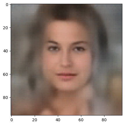
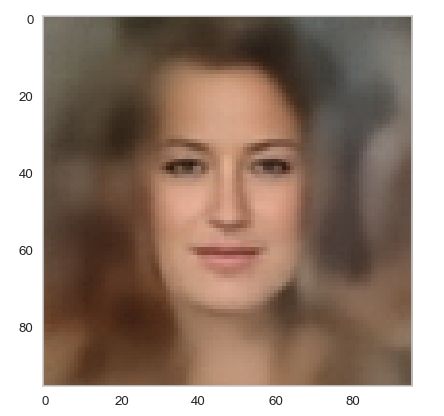
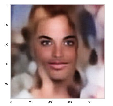
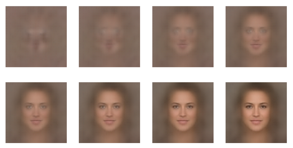
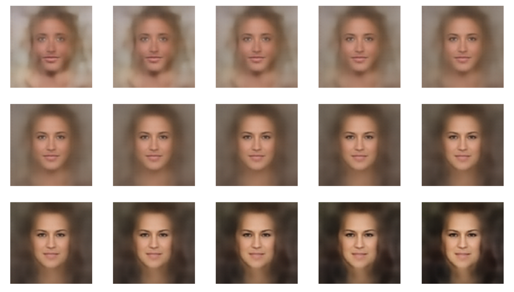
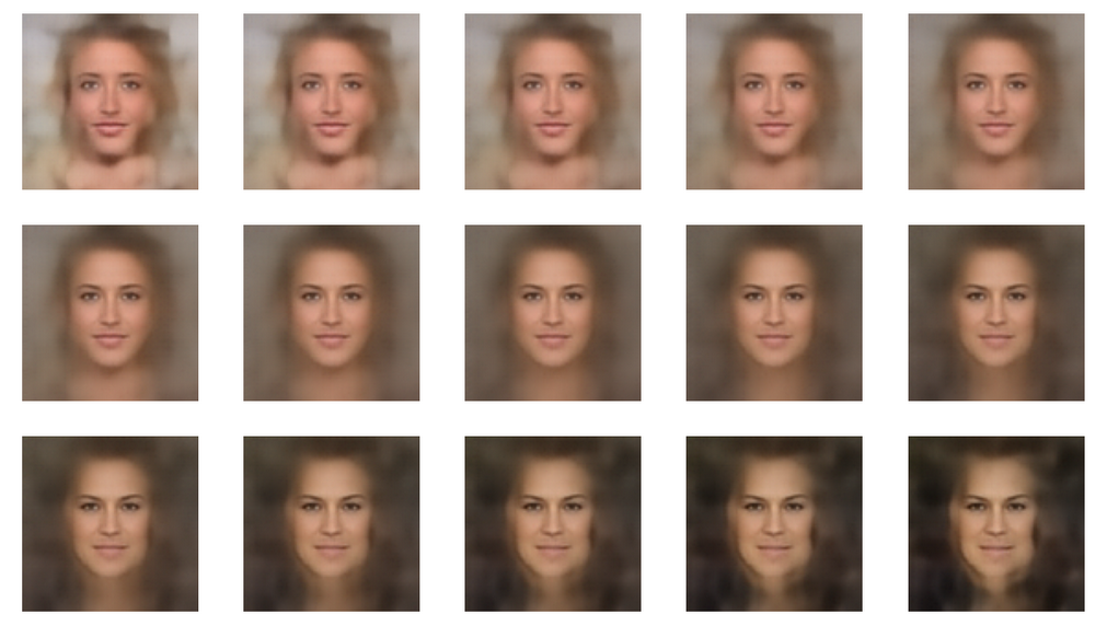
I am going to answer this question in another better prepared post series, soon. To make you a bit curious I leave you with the fact that the following picture shows a face reconstructed by an AE from a randomly selected point in the latent space – with some simple conditions applied: