Post III focused on the shearing of a circle, which was centered in the Euclidean coordinate system [ECS] we worked with. The shear operation resulted in an ellipse with an inclination against the coordinate axes of our ECS. This was interesting regarding four points:
A circle, which is centered in a chosen ECS, exhibits a continuous rotational symmetry (isotropy). This obviously allows for a decomposition of a shear operation into a sequence of two affine operations in the chosen ECS: a scaling operation (with different factors along the coordinate axes) followed by a rotation (or the other way round). Equivalently: We could switch to another specific ECS which is already rotated by a proper angle against our originally chosen ECS and just perform a scaling operation there. The rotation angle is determined by the shear parameter λ. This seems to stand in some contrast to the shearing of figures with only discrete rotational symmetries: We saw for rectangles and cubes that an additional rotation was required to replace the shear operation by a sequence of scaling and rotation operations.
Points (x, y) of circles and ellipses are described by quadratic forms in two dimensions (with some real coefficients α, β, γ, δ):
\[
\alpha \,x^2 \, + \, \beta \, x \, y \, + \, \gamma \, y^2 \:=\: \delta
\]
Quadratic forms play a general role in the mathematical description of cone-sections. (Ellipses are the results of specific cone-sections.)
Ellipses also result from projections of multi-dimensional ellipsoids onto two-dimensional coordinate planes. Multi-dimensional ellipsoids are described by quadratic forms in an ECS covering the ℝn.
Hyper-surfaces for constant probability density values of multivariate normal vector distributions form multi-dimensional ellipsoids. Here we have a link to Machine Learning where key properties of certain objects are often ruled by Gaussian distributions.
From the first point we may expect that a shear operation applied to a multi-dimensional sphere will result in a multi-dimensional ellipsoid – and that such an operation could be replaced by scaling the original sphere (with different factors along n coordinate axes of a n-dimensional ECS) followed by a rotation (or vice versa). We will explicitly investigate this for a 3-dimensional sphere in the next post.
If our assumption were true we would get a first glimpse of the fact that a general multivariate standard distribution can be created by applying a sequence of distinct affine (i.e. linear) operations to a spherical probability distribution. This is discussed in detail in another post-series in this blog.
What is a bit confusing at the moment is that a replacement of a shear operation by simpler affine operations in general seems to require at least two rotations, but only one when we work with centered isotropic bodies. We come back to this point when we discuss the decomposition of a shear matrix by the so called SVD-procedure.
In the previous post of this series we have used the radius of the circle and the shearing parameter λ to derive analytical expressions for the coordinates of special points with extremal values on our ellipse
Points with maximal and minimal y-coordinate values.
Points with a maximal or minimal distance to the symmetry center of the ellipse. I.e. the end-points of the principal diameters of the ellipse.
From the fact that shearing does not change extremal values along the axis perpendicular to the sharing direction we could easily determine the lengths of the ellipse’s principal axes and the inclination angle of the longer axis with the x-axis of our Euclidean coordinate system [ECS].
What do we have in addition? In another mini-series on ellipses
I have meanwhile described how the geometry of an ellipse is related to its quadratic form and respective coefficients of a symmetric matrix. I call this matrix Aq. It forces the components of position vectors to fulfill an equation based on a quadratic polynomial. Furthermore Aq‘s eigenvalues and eigenvectors define the lengths of the ellipse’s principal axes and their inclination to the axes of our chosen ECS. The matrix coefficients in addition allow us to determine the coordinates of the points with extremal y-values on an ellipse. We will use these results later in the present post.
Objectives of this post: Shearing of a centered, rotated ellipse
In this post I want to show that shearing a given centered, but rotated original ellipse EO results in another ellipse ES with a different inclination angle and different sizes of the principal axes.
In addition we will derive the relations of the shearing parameter λS with the coefficients of the symmetric matrix \(\pmb{\operatorname{A}}_q^S \) that defines ES. I also provide formulas for the dependence of ES‘s geometrical properties on the shear parameter λS.
There are two basic prerequisites:
We must show that the application of a shear transformation to the variables of the quadratic form which describes an ellipse EO results in another proper quadratic form and a related matrix \(\pmb{\operatorname{A}}_q^S \).
The coefficients of the resulting quadratic form and of \(\pmb{\operatorname{A}}_q^S \) must fulfill a mathematical criterion for an ellipse.
We expect point 1 to be valid because a shear operation is just a linear operation.
To get some exercise we approach our goals by first looking at the simple case of shearing an axis-parallel ellipse before extending our considerations to general ellipses with an inclination angle against the coordinate axes of our chosen ECS.
This post requires Javascript to display formulas!
A centered, rotated ellipse can be defined by matrices which operate on position-vectors for points on the ellipse. The topic of this post series is the relation of the coefficients of such matrices to some basic geometrical properties of an ellipse. In the previous posts
we have found that we can use (at least) two matrix based approaches:
One reflects a combination of two affine operations applied to a unit circle. This approach led us to a non-symmetric matrix, which we called AE. Its coefficients ((a, b), (c, d)) depend on the lengths of the ellipses’ principal axes and trigonometric functions of its rotation angle.
The second approach is based on coefficients of a quadratic form which describes an ellipse as a special type of a conic section. We got a symmetric matrix, which we called Aq.
We have shown how the coefficients α, β, γ of Aq can be expressed in terms of the coefficients of AE. Another major result was that the eigenvalues and eigenvectors of Aq completely control the ellipse’s properties.
Furthermore, we have derived equations for the lengths σ1, σ2 of the ellipse’s principal axes and the rotation angle by which the major axis is rotated against the x-axis of the Cartesian coordinate system [CCS] we work with.
We have also found equations for the components of the position vectors to those points of the ellipse with maximum y-values.
In this post we determine the components of the vectors to the end-points of the ellipse’s principal axes in terms of the coefficients of Aq. Afterward we shall test our formulas by a Python program and plots for a specific example.
Reduced matrix equation for an ellipse
Our centered, but rotated ellipse is defined by a quadratic form, i.e. by a polynomial equation with quadratic terms in the components xe and ye of position vectors to points on the ellipse:
The quadratic polynomial can be formulated as a matrix operation applied to position vectors vE = (xE, yE)T. With the the quadratic and symmetric matrix Aq
Method 1 to determine the vectors to the principal axes’ end points
My readers have certainly noticed that we have already gathered all required information to solve our task. In the first post of this series we have performed an eigendecomposition of our symmetric matrix Aq. We found that the two eigenvectors of Aq for respective eigenvalues λ1 and λ2 point along the principal axes of our rotated ellipse:
This is trivial regarding the algebraic operations, but results in lengthy (and boring) expressions in terms of the matrix coefficients. So, I skip to write down all the terms. (We do not need it for setting up ordered numerical programs.)
Remember that you could in addition replace (α, β, γ) by coefficients (a, b, c, d) of matrix AE. See the first post of this series for the formulas. This would, however, produce even longer equation terms.
We pick the yE with the positive term in the following steps. (The way for the solution with the negative term in yE is analogous.) The square of yE is:
A detailed analysis also for the other yE-expression (see above) leads to further solutions for the coordinates (=vector component values) of points with extremal values for the radii. These are the end-points of the principal axes of the ellipse:
I leave it to the reader to expand the convenience variables into terms containing the original coefficients α, β, γ.
Plots
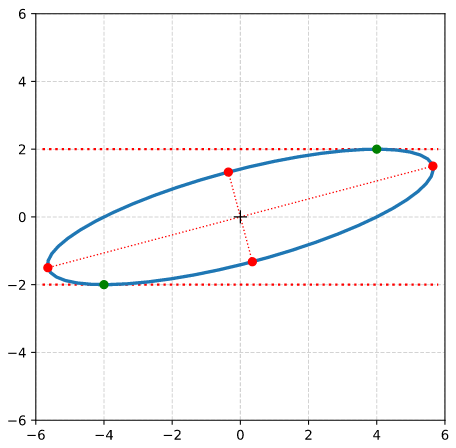
It is easy to write a Python program, which calculates and plots the data of an ellipse and the special points with extremal values of the radii and extremal values of ye. The general steps which I followed were:
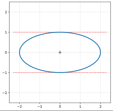
Step 0: Create 100 points a unit circle. Save the coordinates in Python lists (or Numpy arrays). Use Matplotlib’s plot(x,y)-function to plot the vectors.
Step 1: Create an axis-parallel ellipse with values for the axes ha = 2.0 and hb = 1.0 along the x- and the y-axis of the Cartesian coordinate system [CCS]. Do this by applying a diagonal scaling matrix Dσ1, σ2 (see the first post of this series).
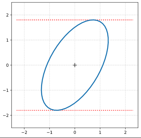
Step 2: Rotate the ellipse bei π/3 (60 °). Do this by applying a rotation matrix Rπ/3 to the position vectors of your ellipse (with the help of Numpy). Alternatively, you can first create the matrices, perform a matrix multiplication and then apply the resulting matrix to the position vectors of your unit circle.
(The limiting lines have been calculated by the formulas given above.)
Step 3: Determine the coefficients of combined matrix AE = Rπ/3 ○ Dσ1, σ2
I got for the coefficients ( (a, b), (c, d) ) of AE :
A_ell =
[[ 1.         -0.8660254 ]
[ 1.73205081  0.5       ]]
Step 3: Determine the coefficients of the matrix Aq by the formulas given in the first post of this series. I got
A_q =
[[ 3.25       -1.29903811]
[-1.29903811  1.75      ]]
For δ I got:
delta = 4.0
which is consistent with the length-values of the principal axes.
Step 4: Determine values for the eigenvalues λ1 and λ2 from the Aq-coefficients by the formulas given in the first post. Also calculate them by using Numpy’s
eigenvalues, eigenvectors = numpy.linalg.eig(A_q). Theory tells us that these values should be exactly λ1 = 4 and λ1 = 1. I got
Eigenvalues from A_q: lambda_1 = 4. :: lambda_2 = 1.
Step 5: Determine the components of the normalized eigenvectors with the help of numpy.linalg.eig(A_q). I got:
Components of normalized eigenvectors by theoretical formulas from A_q coefficients:
ev_1_n :  -0.8660254037844386  :  0.5000000000000002
ev_2_n :  0.5000000000000001  :  0.8660254037844385

Eigenvectors from A_q via numpyy.linalg.eig():
ev_1_num :  0.8660254037844387  :  -0.5000000000000001
ev_2_num :  0.5000000000000001  :  0.8660254037844387
The deviation between ev_1_n and ev_1_num is just due to a difference by -1. This is correct as the eigenvectors are unique only up to a minus-sign in all components.
Step 6: Calculate the sinus of the rotation angle of our ellipse from Aq– and Aq-coefficients. The theoretical value is sin(2 π/3) = sin(2 pi/3) = 0.8660254037844387. I got:
sin(2. * rotation angle) of major axis of the ellipse against the CCS x-axis from A_E coefficients:
sin_2phi-A_E  =  0.8660254037844388

sin(2. * rotation angle) of major axis of the ellipse against the CCS x-axis from from eigenvectors of A_q:
sin_2phi-ev_A_q =  0.8660254037844387

sin(2. * rotation angle) of major axis of the ellipse against the CCS x-axis from A_q-coefficients:
sin_2phi-coeff-A_q =  0.8660254037844388
Perfect!
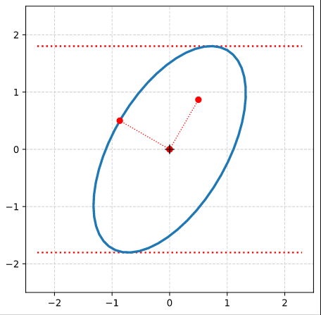
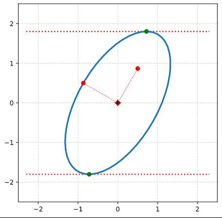
Step 7: Plot the end-points of the normalized eigenvectors of Aq:
Note that in our example case the end-point of the eigenvector along the minor axis must be located exactly on the elliptic curve as the ellipses minor axes has a length of b=1!
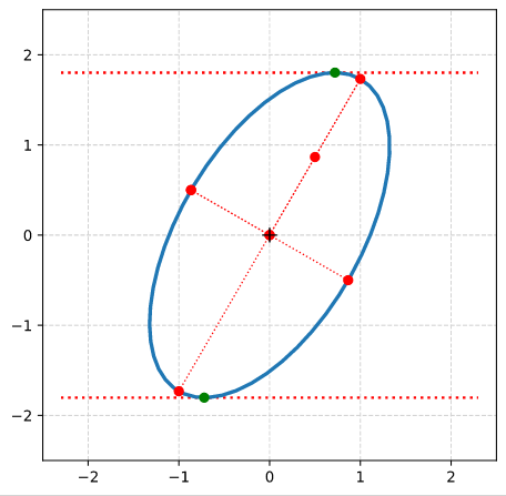
Step 8: Calculate the components of the vectors to data-points of the ellipse with maximal absolute ye-values from the Aq-coefficients given in the previous post. Plot these data-points (here in green color).
Step 9: Calculate the components of the vectors to data-points of the ellipse with maximal values of the radii with the help of the complex formulas presented in this post and plot these points in addition.
Conclusion
In this mini-series of posts we have performed some small mathematical exercises with respect to centered and rotated ellipses. We have calculated basic geometrical properties of such ellipses from the coefficients of matrices which define ellipses in algebraic form. Linear Algebra helped us to understand that the eigenvectors and eigenvalues of a symmetric matrix, whose coefficients stem from a quadratic equation (for a conic section), control both the orientation and the lengths of the ellipse’s axes completely.
This knowledge is useful in some Machine Learning [ML] context where elliptic data appear as projections of multivariate normal distributions. Multivariate Gaussian probability functions control properties of a lot of natural objects. Experience shows that certain types of neural networks may transform such data into multivariate normal distributions in latent spaces. An evaluation of the numerical data coming from such ML-experiments often delivers the coefficients of defining matrices for ellipses.
In my blog I now return to the study of with shearing operations applied to circles, spheres, ellipses and 3-dimensional ellipsoids. Later I will continue with the study of multivariate normal distributions in latent spaces of Autoencoders. For both of these topics the knowledge we have gathered regarding the matrices behind ellipses will help us a lot.
This post requires Javascript to display formulas!
Convolutional Autoencoders and multivariate normal distributions
Experiments as with my own on convolutional Autoencoders [CAE] show: A CAE maps a training set of human face images (e.g. CelebA) onto an approximate multivariate vector distribution in the CAE’s latent space Z. Each image corresponds to a point (z-point) and a corresponding vector (z-vector) in the CAE’s multidimensional latent space. More precisely the results of numerical experiments showed:
The multidimensional density function which describes the inner dense core of the z-point distribution (containing more than 80% of all points) was (aside of normalization factors) equivalent to the density function of a multivariate normal distribution[MND] for the respective z-vectors in an Euclidean coordinate system.
After a normalization with an appropriate factor the continuous density functions controlling the multivariate vector distribution can be interpreted as a probability density function [p.d.f.]. The components vj (j=1, 2,…, n) of the vectors to the z-points are regarded as logically separate, but not uncorrelated variables. For each of these variables a component specific value distribution Vj is given. All these marginal distributions contribute to a random vector distribution V, in our case with the properties of a MND:
μ is a vector with all mean values μj of the Vj component distributions as its components. Σ abbreviates the covariance matrix relating the distributions Vj with one another.
The point distribution of a CAE’s MND forms a complex rotated multidimensional ellipsoid with its center somewhere off the origin in the latent space. The latent space itself typically has many dimensions. In the case of my numerical experiments the number of dimension was n ≥ 256. The number of sample vectors used were between 80,000 and 200,000 – enough data to approximate the vector distribution by a continuous density function. The densities for the Vj-distributions formed a smooth Gaussian function (for a reasonable sampling interval). But note: One has to be careful: The fact that the Vj have a Gaussian form is not a sufficient condition for a MND. (See the next post.) But if a MND is given all Vj have a Gaussian form.
Generative use of MNDs in multidimensional latent spaces of high dimensionality
When we want to use a CAE as a generative tool we need to solve a problem: We must create statistical vectors which point into the (multidimensional) volume of our point distribution in the latent space of the encoding algorithm. Only such vectors provide useful information to the Decoder of the CAE. A full multivariate normal distribution and hyperplanes of its multidimensional density function are difficult to analyze and to control when developing a proper numerical algorithm. Therefore I want to reduce the problem of vector generation to a sequence of viewable and controllable 2-dimensional problems. How can this be achieved?
A central property of a multivariate normal distribution helps: Any sub-selection of m vector-component distributions forms a multivariate normal distribution, too (see below). For m=2 and for vector components indexed by (j,k) with respective distributions Vj, Vk we get a so called “bivariate normal distribution” [BND]:
for vector component values vj, vk defines a point density of the sample data in the (j,k)-coordinate plane of the Euclidean coordinate system in which the MND is described. The density function of the marginal distributions Vj showed the typical Gaussian forms of a univariate normal distribution.
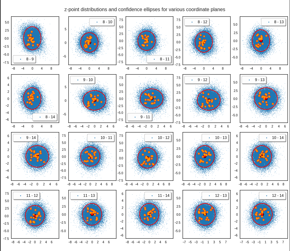
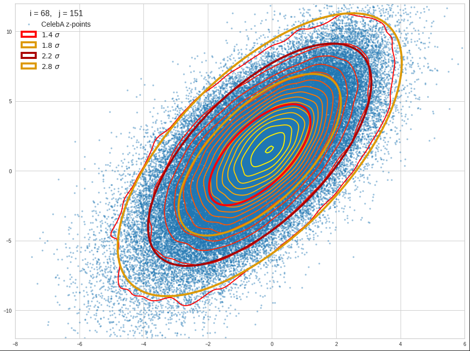
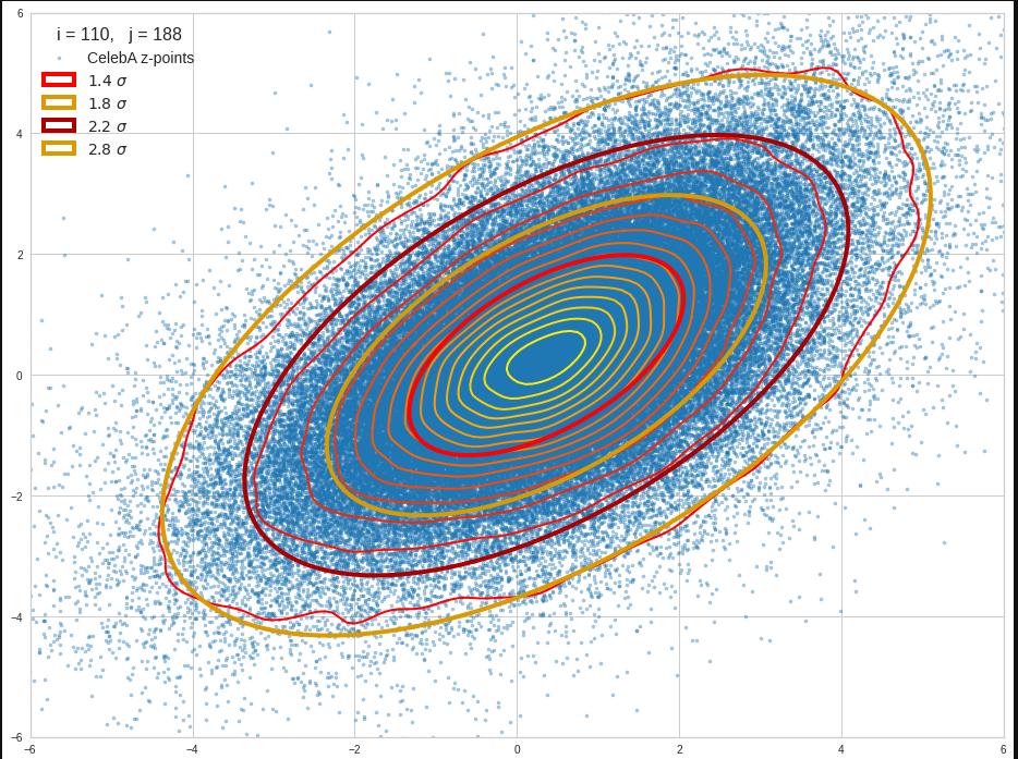
The density function of a BND has some interesting mathematical properties. Among other things: The hyperplanes of constant density of a BND’s density function form ellipses. This is illustrated by the following plots showing such contour lines for selected pairs (Vj, Vk) of a real point-distribution in a 256-dimensional latent space. The point distribution was created by a CAE in its latent space for the CelebA dataset.
Contour lines for selected (j,k)-pairs. The thick lines stem from theory and calculated correlation coefficients of the univariate distributions.
The next plot shows the contours of selected vector-component pairs after a PCA-transformation of the full MND. (Main ellipse axes are now aligned with the axes of the PCA-coordinate system):
These ellipses with axes along the coordinate axes are relatively easy to handle. They can be used for vector creation. But they require a full PCA transformation of the MND-distribution, a PCA-analysis for complexity reduction and an application of the inverse PCA-transformation. The plot below shows the point-density compared to a 2.2-σ-confidence ellipses. The orange points are the results of a proper statistical numerical vector generation algorithm based on a PCA-transformation of the MND.
See my post quoted above for the application of a PCA-transformation of the multidimensional MND for vector creation.
However, we get the impression that we could also use these rotated ellipses in projections of the MND onto coordinate planes of the original latent space system directly to impose limiting conditions on the component values of statistical vectors pointing to an inner regions of the MND. Of course, a generated statistical vector must then comply with the conditions of all such ellipses. This requires an analysis and combined use of the ellipses of all of the subordinate BNDs of a the original MND during an iterative or successive definition of the values for the vector components.
Objective of this post series
In my last post about CAEs (see the link given above) I have explicitly asked the question whether one can avoid performing a full PCA-transformation of the MND when creating statistical vectors pointing to a defined inner region of a MND.
The objective of this post series is to prove the answer: Yes, we can. And we will use the BNDs resulting from projections of the original MND onto coordinate planes. We will in particular explore the n*(n-1)/2 the properties of the BNDs’ confidence ellipses. As said: These ellipses are rotated against the coordinate system’s axes. We will have to deal with this in detail. We will also use properties of their 1-dimensional marginal distributions (projections onto the coordinate axes, i.e. the Vj.)
In addition we need to prepare a variety of formulas before we are able to define numerical procedure for the vector generation without a full PCA-transformation of the MND with around 100,000 vectors. Some of the derived formulas will also allow for a deeper insight into how the multiple BNDs of a MND are related between each other and with confidence hypersurfaces of the MND.
Ellipses in general lead to equations governed by quadratic or fourth power polynomials. We will in addition use some elementary correlation formula from statistics and for some exercises a simple optimization via derivatives. The series can be regarded as an excursion into some of the math which governs bivariate distributions resulting from a MND.
As MNDs may also be the result of other generative Machine Learning algorithms in respective latent spaces, the whole approach to statistical vector generation for such cases should be of general interest. Note also that the so called “central limit theorem” almost guarantees the appearance of MNDs in many multivariate datasets with sufficiently large samples and value dependencies on many singular observations.
Distributions of a variety of variables may result in a MND if the variables themselves depend on many individual observables with limited covariance values of their distributions. In particular pairwise linearly correlated Gaussian density distributions individual variables (seen as vector components) may constitute a MND if the conditional probabilities fulfill some rules. We will see a glimpse of this in 2 dimensions when we analyze integrals over Gaussians in the bivariate normal case.
Other approaches to statistical vector generation?
Well, we could try to reconstruct the multidimensional density function of the MND. This is a challenge which appears in some problems of pure statistics, but also in experimental physics. See e.g. a paper of Rafey Anwar, Madeline Hamilton, Pavel M. Nadolsky (2019, Department of Physics, Southern Methodist University, Dallas; https://arxiv.org/pdf/1901.05511.pdf). Then we would have to find the elements of the (inverse) covariance matrix or – equivalently – the elements of a multidimensional rotation matrix. But the most efficient algorithms to get the matrix coefficients again work with projections onto coordinate planes. I prefer to use properties of the ellipses of the bivariate distributions directly.
Note that using the multidimensional density function of the MND directly is not of much help if we want to keep the vectors’ end points within a defined multidimensional inner region of the distribution. E.g.: You want to limit the vectors to some confidence region of the MND, i.e. to keep them inside a certain multidimensional ellipsoidal contour hyper-surface. The BND-ellipses in the coordinate planes reflect the multidimensional ellipsoidally shaped contour hyperplanes of the full distribution. Actually, when we vertically project a multidimensional hyperplane onto a coordinate plane then the outer 2-dim border line coincides with a contour ellipse of the respective BND. (This is due to properties of a MND. We will come back to this in a future post.) The problem of proper limiting individual vector component values thus again is best solved by analyzing properties of the BNDs.
Steps, methods, mathematical level
As a first step I will, for the sake of completeness, write down the formula for a multivariate normal distribution, discuss a bit its mathematical construction from uncorrelated univariate normal distribution. I will also list up some basic properties of a MND (without proof!). These properties will justify our approach to create statistical vectors pointing into a defined inner region of the MND by investigating projected contour ellipses of all subordinate BNDs. As a special aspect I want to make it at least plausible, why the projected contour ellipses define infinitesimal regions of the same relative probability level as their multidimensional counterparts – namely the multidimensional ellipsoidal hypersurfaces which were projected onto coordinate planes.
Then as a first productive step I want to motivate the specific mathematical form of the probability density function [p.d.f] of a bivariate normal distribution. In contrast to many of the math papers I have read on the topic I want to use a symmetry argument to derive the basic form of the p.d.f. I will point out an important, but plausible assumption about conditional distributions. An analogous assumption on the multidimensional level is central for the properties of a MND.
As the distributions Vj and Vk can be correlated we then want to understand the impact of the correlation coefficients on the parameters of the 2-dimensional density function. To achieve this I will again derive the density function by using our previous central assumption and some simple relations between the expectation values of the constituting two univariate distributions in the linear correlation regime. This concludes the part of the series where we get familiar with BNDs.
Furthermore we are interested in features and consequences of the 2-dimensional density functions. The contour lines of the 2-dim density function are ellipses – rotated by some specific angle. I will look at a formal mathematical process to construct such ellipses – in particular confidence ellipses. I will refer to the results Carsten Schelp has provided in an Internet article on this topic.
His construction process starts with a basic ellipse, which I will call base correlation ellipse[BCE]. The length of the axes of this ellipse are eigenvalues of the covariance matrix of the standardized marginal distributions constituting the BND. The main axes of this elementary ellipse are in addition aligned with the two selected axes of a basic Euclidean coordinate system in which the bivariate distribution is defined. The length of the BCE’s main axes can be shown to depend on the correlation coefficient for the two vector component distributions Vj and Vk. This coefficient also appears in the precision matrix of the BND. Points on the base correlation ellipse can be mapped with two steps of an affine transformation onto points on the real contour ellipses, in particular to points of the confidence ellipses.
The whole construction process is not only of immense help when designing visualization programs for the contour ellipses of our distribution with many (around 100,000) individual vectors. The process itself gives us some direct geometrical insights. It also helps to avoid finding a numerical solution of the usual eigenvector-problems when answering some specific questions about the rotated contour ellipses. Normally we solve an eigenvalue-problem for the covariance matrix of the multi- or the many subordinate bi-variate distributions to get precise information about contour ellipses. This corresponds to a transformation of the distributions to a new coordinate system whose axes are aligned to the main axes of the ellipses. Numerically this transformation is directly related to a PCA transformation of the vector distributions. However, such a PCA-transformation can be costly in terms of CPU time.
Instead, we only need a numerical determination of all the mutual the correlation coefficients of the univariate marginal distributions of the MND. Then the eigenvalue problem on the BND-level is already analytically solved. We therefore neither perform a full numerical PCA analysis of the MND and multidimensional rotation of the vectors of around 100,000 samples. Nor do we analyze explained variance ratios to determine the most important PCA components for dimensionality reduction. We neither need to perform a numerical PCA analysis of the BNDs.
Most important: Our problem of vector generation is formulated in the original latent space coordinate system and it gets a direct solution there. The nice thing is that Schelp’s construction mechanism reduces the math to the solution of quadratic polynomial equations for the BNDs. The solutions of those equations, which are required for our ultimate purpose of vector generation, can be stated in an explicit form.
Therefore, the math in this series will mostly remain on high school level (at least at a level given when I was young). Actually, it was fun to dive back into exercises reminding me of school 50 years ago. I hope the interested reader has some fun, too.
Solutions to some particular problems with respect to the confidence ellipses of the MND’s BNDs
In particular we will solve the following problems:
Problem 1: The two points on the BCE-ellipse with the same vj-value are not mapped onto points with the same vj-value on the confidence ellipse. We therefore derive the coordinates of points on the BCE-ellipse that give us one and the same vj-value on the real confidence ellipse.
Problem 2: Plots for a real MND vector distribution indicate that all (n-1) confidence ellipses of distribution pairs of a common Vj with other marginal distributions Vk (for the same confidence level and with k ≠ j) have a common tangent parallel to one coordinate axis. We will derive the value of a maximum v_j-value for all ellipses of (j,k)-pairs of vector component distributions. We will prove that it is identical for all k. This will define the common interval of allowed vj-component-values for a bunch of confidence ellipses for all (Vj, Vk)-pairs with a common Vj.
Problem 3: The BCE-ellipses for a common j-, but different k-values depend on different values for the correlation coefficients ρj,k of Vj with its various Vk counterparts. Therefore we need a formula that relates a point on the BCE-ellipse leading to a concrete v_j-value of the mapped point on the confidence ellipse of a particular (Vj, Vk)-pair to respective points on other BCE-ellipses of different (Vj, Vm)-pair with the same resulting v_j-value on their confidence ellipses. I will derive such a formula. It will help us to apply multiple conditions onto the vector component values.
Problem 4: As a supplemental exercise we will derive a mathematical expression for the size of the main axes and the rotation angle of the ellipses. We should, of course, get values that are identical to results of the eigenwert-problem for the correlation matrix (describing a PCA coordinate transformation). This gives us additional confidence in Schelps’ approach.
In the end we can use our results to define a numerical algorithm for the direct creation of vectors pointing to a defined inner region of the multivariate normal distribution. As said, this algorithms does not require a costly PCA transformations of the full MND or many, namely n*(n-1)/2 such PCA-transformations of its BNDs.
I intend to visualize all results with the help of a concrete example of a multivariate example distribution created by a CAE for the CelebA dataset. The plots will use Schelp’s construction algorithm for the confidence ellipses extensively.
Conclusion and outlook
Convolutional Autoencoders create approximate multivariate normal distributions [MND] for certain input data (with Gaussian pattern properties) in their latent space. MNDs appear in other contexts of machine learning and statistics, too. For evaluation and generative purposes one may need statistical vectors with end points inside a defined multidimensional hypersurface corresponding to a certain confidence level and a certain constant density value of the MND’s density function. These hypersurfaces are multidimensional ellipsoids.
We have the hope that we can use mathematical properties of the MND’s subordinate bivariate normal distributions [BNDs] to create statistical vectors with end points inside the multidimensional confidence ellipsoids of a MND. Typically such an ellipsoid resides off the origin of the latent space’s coordinate system and the ellipsoid’s main axes are rotated against the axes of the coordinate system. We intend to base the confining conditions on the components of the aspired statistical vectors on correlation coefficients of the marginal vector component distributions. Our numerical algorithm should avoid a full PCA-transformation of the multidimensional vector distribution.
In the next post of this series I give a formula for the density function of a multivariate normal distribution. In addition I will list up some basic properties which justify the vector generation approach via bivariate normal distributions.
My present post series explores options to use a standard convolutional Autoencoder [AE] for the creation of images with human faces. The face generation should based on random input to the AE’s Decoder. On our quest for a suitable method we have meanwhile learned a lot about other aspects of Autoencoders, vector distributions in multi-dimensional latent spaces and generative methods for our special case:
Methods to create statistical latent vectors [z-vectors] as input for the AE’s Decoder must be chosen carefully. Among other things: It is difficult to create a bunch of random vectors which cover wider areas in the vastness of a multidimensional space. So the z-vector creation must be adjusted to specific requirements.
After having been trained with CelebA images a convolutional AE fills a limited and coherent region in the latent space with z-points for the training images. This latent space region appears to be critical for successful image creation: Statistically generated z-vectors should point to this region. The core of the z-point distribution gets filled relatively densely.
A convolutional AE maps human face images onto an approximate multivariate normal distribution. This gives the inner core of the z-point distribution the structure of a multidimensional ellipsoid. The projections of this ellipsoid onto 2-dimensional coordinate planes show characteristic nested elliptic contour lines.
As the main axes of these ellipses were inclined with different angle towards the axes of chosen coordinate planes we concluded that linear correlations mark average dependencies between the z-vector components. Limiting conditions imposed by these correlations must also be fulfilled by z-vectors used as the Decoder’s input.
See previous posts in this series for more details. In particular, the last 2 posts
have shown that the density distribution for the z-points really exhibits elliptic contour lines in the original coordinate system of the latent space and(!) in the target coordinate system of a PCA transformation.
In this post we use our gathered knowledge: I present a first simple method to generate z-vectors which point to the latent space region filled by z-points for CelebA images. These z-vectors will fulfill the general and limiting elliptic conditions for their components.
Decomposing the full problem of latent vector generation into a sequence of 2-dimensional problems
The nice thing about multivariate Gaussian distributions with linear correlations between the vector components is the following: We can reduce the problem of choosing proper component values to a series of 2-dimensional restrictions. Firstly we can use characteristic properties of the Gaussian distribution for each component. And secondly we can use confidence ellipses in 2-dimensional coordinate planes to restrict the component values to allowed intervals.
Ellipses are most easy to handle when their axes are aligned with the axes of the coordinate system in which we describe them. So, let us assume that we know an affine transformation T to a new coordinate system which also has orthogonal axes and supports the following special transformation properties for a multivariate normal density distribution:
T maps nested elliptic contour lines of the multidimensional density distribution and in particular confidence ellipses for component pairs in the original coordinate system to nested elliptic contours and confidence ellipses in the new coordinate system.
Taligns the centers of the transformed ellipses with the origin of the new coordinate system.
T aligns the main axes of the mapped ellipses with the axes of the new coordinate system.
T is reversible.
How could we then use the transformed data for vector-creation?
In the new coordinate system, a contour ellipse in a chosen coordinate plane for the axes-indices (i, j) may have main diameters of size
d1 = 2 * a and d2 = 2 * b.
We then can first select a randomv_i value to fall into a range [-a * fact, a * fact].
– fact * a < v_i < fact * a
With fact being a proper factor. This factor defines a confidence level in the new coordinate system. With the value of v_i fixed and b being the half-diameter in the orthogonal direction the correlation condition for the z-point distribution says that the v_j value must fall into an interval [-c, c] defined by:
-c < v_j < c, with c = b * fact * sqrt(1 – x**2 / (fact * a)**2)
But within these limits we can again choose the v_j-value freely. Below I use a simple random-function for a constant probability density to pick a value.
However: It would not be enough to restrict the coordinates to the conditions of just one ellipse! The components of the created vectors must in parallel fulfill elliptic conditions for all of the possible pairs of vector-components. I.e. we may need to adapt the v_j values gained from the analysis of a fist 2D-ellipse to further conditions of other ellipses and component pairs. This can be achieved by an iteration. For z_dim = 256 this involves a total of 32640 checks and possible value-adaptions to each and all of the allowed value ranges.
In addition: The order by which the component-pairs and their conditions are investigated must be randomized to get real statistical vector distributions.
Eventually the resulting vector components must be re-transformed into the original coordinate system of the latent space.
The ellipse for the “core’s boundary” in the original coordinate system will be defined by the chosen confidence level of the ellipsoidal normal distribution. We saw already that a confidence level of σ = 2.0 defines the transition to outer regions of the z-point density distribution quite well.
This all sounds manageable by relative simple Python programs. But: Do we know a proper transformation T? Yes, we do: A PCA-transformation of the z-point density distribution has all the properties discussed above.
Using half maximum values after a PCA transformation of the z-point distribution
The last post proved that a PCA transformation maps ellipses onto ellipses for component pairs in the transformed PCA coordinate system. The advantage of the ellipses there is that their main axes are on average well aligned with the orthogonal PCA coordinate axes. Gaussians for the number density distribution per component are mapped to Gaussians for the new components in the transformed coordinate system. So, the basic idea for a proper z-vector generation is:
Take the multivariate normal z-point distribution for the training images in the AE’s latent space.
Apply a PCA analysis to diagonalize the correlation matrix and transform the z-vector components to the PCA coordinate system.
Use the ellipses in coordinate planes of the PCA coordinate system to create random z-vector components fulfilling all required conditions there.
Re-transform the resulting z-vector components into the original coordinate system of the latent space.
Point 3 in our method is covered by a numerical analysis of the Gaussians in the PCA-coordinate system. We determine the half-width numerically by analyzing the density distribution with the help of sampling intervals. This simple method has resolution limits related to the size of the sampling interval. This has consequences for PCA components with a small standard deviation. We saw already in the last posts that such distributions appear for higher PCA components at the lower end of the explained variance.
Does the suggested method work?
The convolutional AE we work with was defined in previous posts with 4 Conv2D layers in the Encoder and 4 Conv2DTranspose layers in Decoder. The number of latent space dimensions was z_dim = 256. The AE network was trained on CelebA images. I do not want to bore you with details of the codes for the creation of z-vectors consistent to the resulting elliptic conditions. It is all standard. The PCA-transformation can e.g. be taken from the sklearn-package.
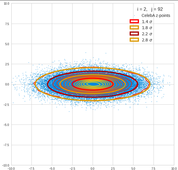
I have applied a constant probability density to choose a random value within the allowed ranges for the component values of the aspired z-vectors in the PCA coordinate system. For the plots below I have used the most important 50 to 105 PCA components (out of 256). The plots include confidence ellipses on a level of σ = 2.2. I derived the confidence ellipses by directly evaluating the standard deviations of the transformed distribution data in all coordinate directions.
The first plot shows you such an ellipse for the coordinate plane corresponding to the first two, most important PCA components. The orange points mark 20 z-points defined by 20 randomly z-vectors fulfilling all elliptic conditions. The plot contains 120,000 z-points for images out of the 170,000 CelebA pictures used during training.
Generated statistical vectors in the PCA coordinate system
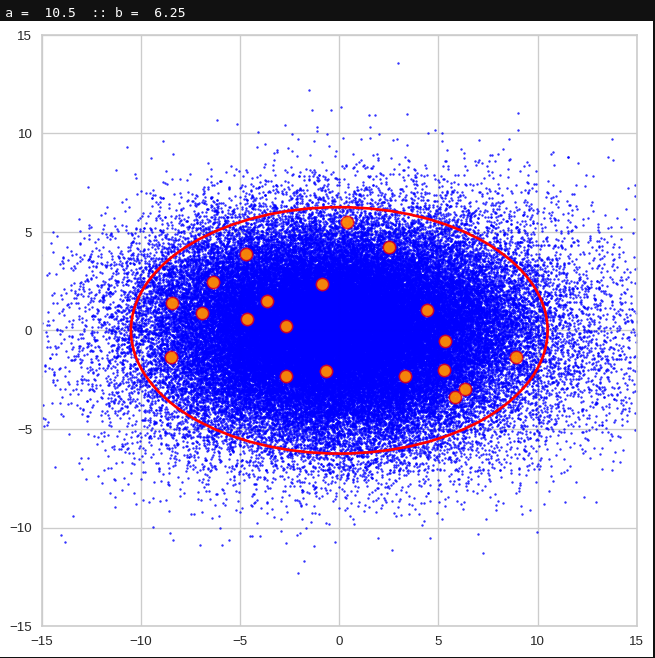
For elliptic contour lines see the last post before the present one in this series. The next plot shows the same generated 20 z-vectors for other component-combinations among the first 20 of the most important PCA-components. The plots contain a selection of 60,000 z-points.
The outer z-points points do not always indicate that we have elliptic contours in the denser core of the displayed 2-dimensional distributions. But see the last post for proofs that the inner core inside the red ellipse really displays elliptic contours. You see that all random vectors lie within the 2-σ-ellipses.
The next plot shows the generated z-vectors in the original coordinate system of the latent space. The component values were back-transformed from the PCA-system to the original coordinate system.
Generated statistical z-vectors after an inverse PCA transformation to the original coordinate system of the latent space
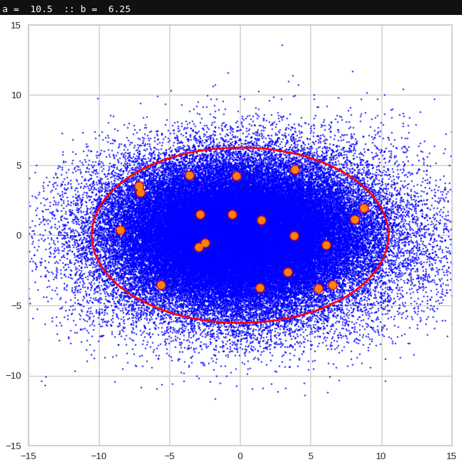
We get similar plots for other component pairs. And of course for other generated vectors.
Generated statistical z-vectors in the PCA coordinate system
Generated statistical z-vectors after an inverse PCA transformation to the original coordinate system of the latent space
Technically we have obviously achieved what we wanted: Our generated statistical vectors are distributed within the core of our multidimensional ellipsoid.
Note that this method fortunately works even when we use a limited number of the PCA components, only. This is due to intricate properties of a PCA transformation which guarantee that a back-transformation puts the resulting points close to the original ones even when we omit less important PCA components. I cannot discuss the math-details in this blog. You have to see scientific literature for this. An introduction is e.g. provided by https://arxiv.org/pdf/1404.1100.pdf.
For me this property of the PCA transformation was helpful when I ran into the resolution problem for a proper half-width of the Gaussians. Taking 256 components lead to errors as elliptic conditions for very narrow Gaussians were not properly defined and some of the created vectors left the allowed value ranges.
Resulting face images
Let us look at some results. First I want to remind you from where we started:
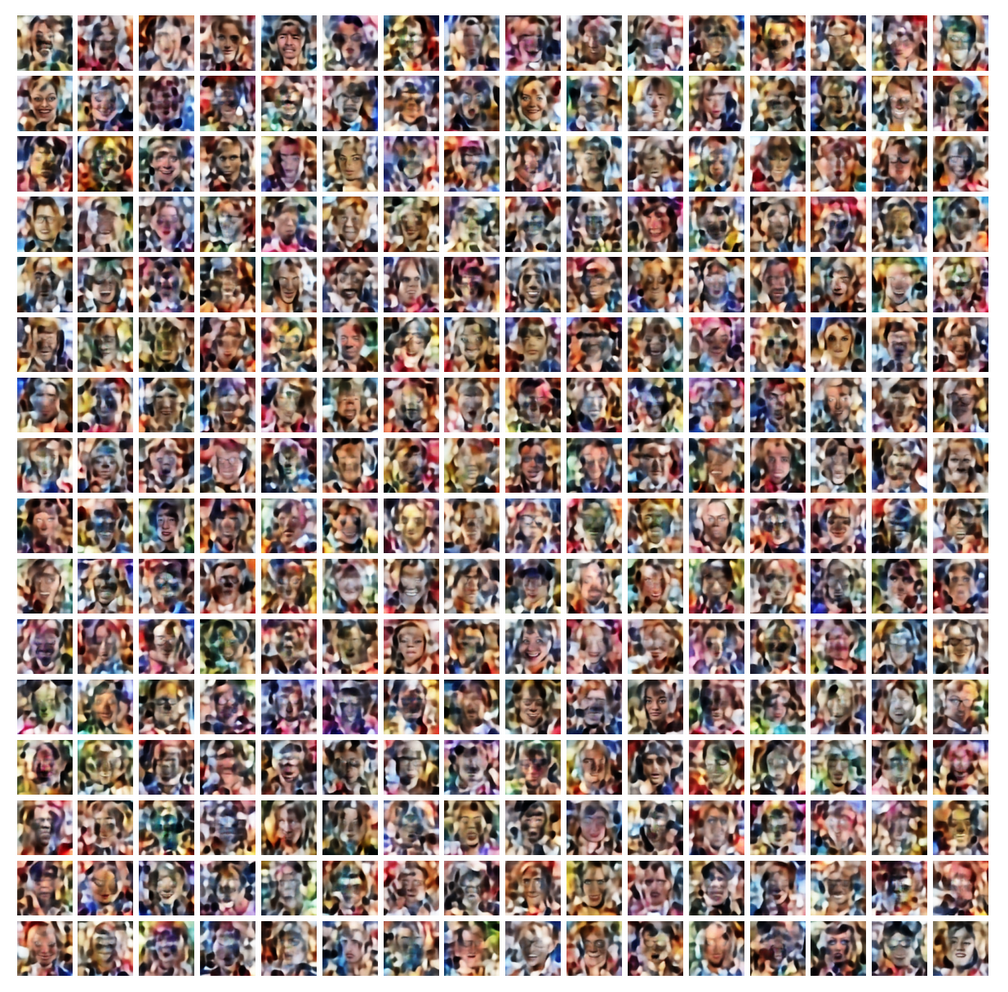
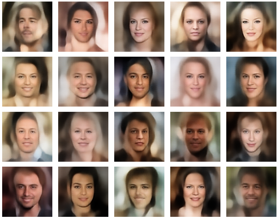
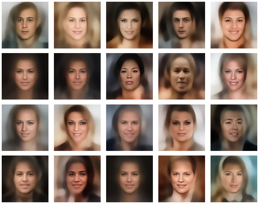
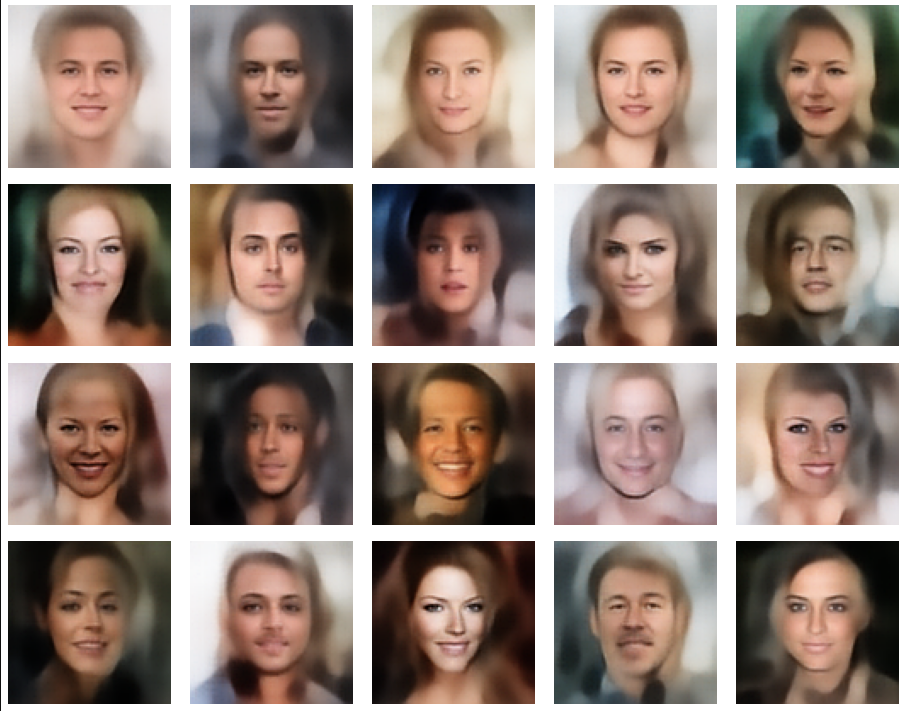
Failed trials with improper random z-vectors based on constant probability densities
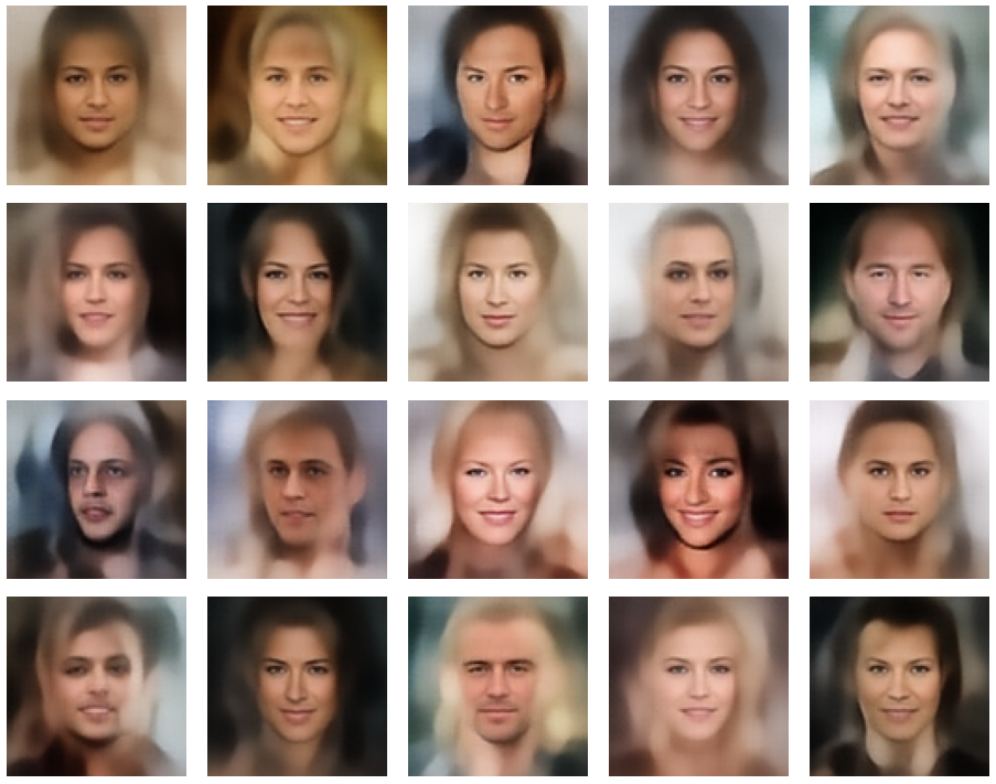
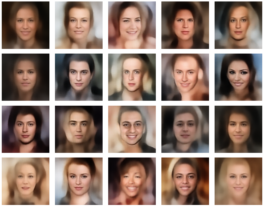
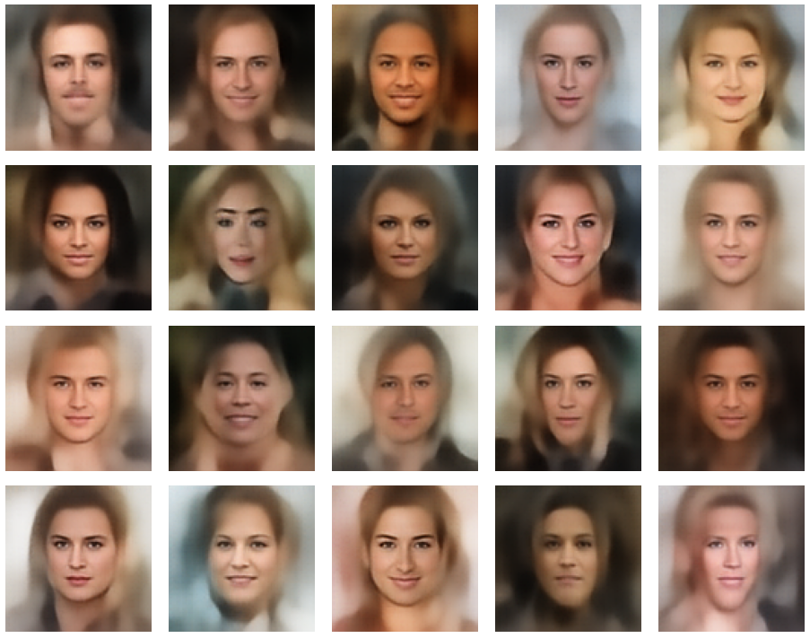
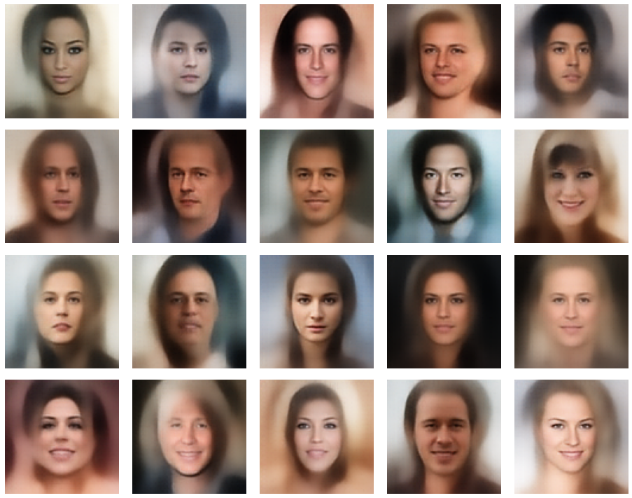
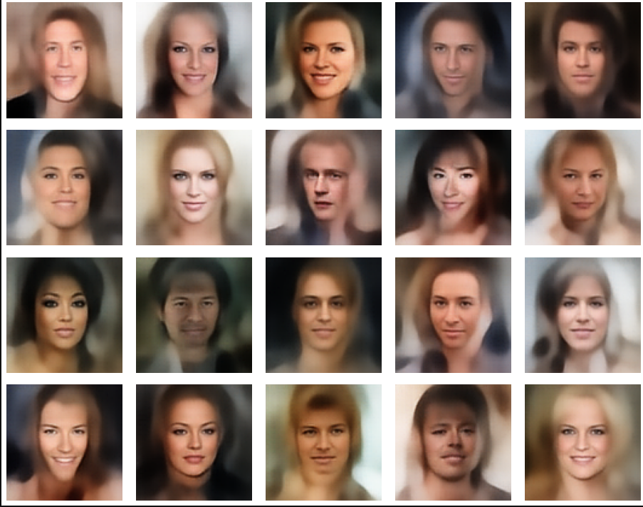
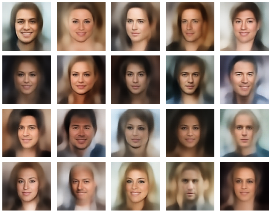
A simple random generator used in the beginning was totally inapt to feed the AE’s Decoder with proper statistical z-vectors. And now – look at the following plots. They were produced for a varying number of PCA components between 50 and 120, 100000 statistically selected z-points within a 3 σ-level for the PCA-transformation and various factors 0.6 < fact < 0.8 used upon a half-width corresponding to a confidence level of 2.35 σ:
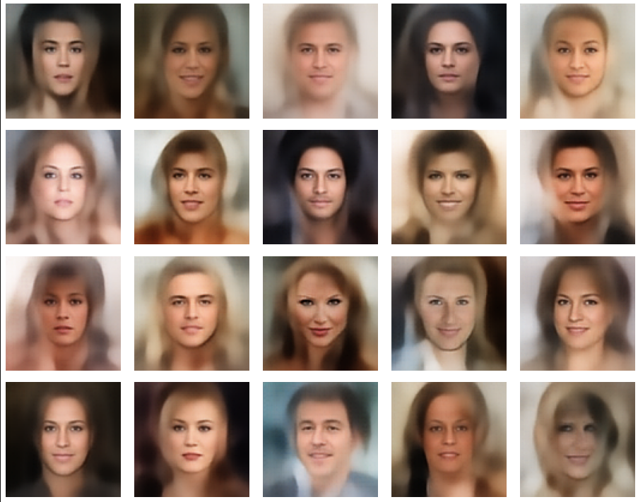
In some cases – for a higher number of PCA components – we even see smaller details of the face images and a reasonable transition to some kind of hairdo. Please remember that z_dim = 256 is a pretty low number for the latent space to cover the encoding of face details. And celebrities as covered by CelebA use make-up ….
In case you think the above result is not noteworthy: Please remember that we talk about a simple standard Autoencoder and not about a Variational Autoencoder and neither about a transformer based Autoencoder. No fancy additions to cost functions or special layers. And who ever has read the very instructive book of D. Foster on “Generative Deep Learning” (1st edition, O’Reilly) may compare his images to mine. And I have used a lower resolution of the original images than D. Foster. Just to motivate people to look a bit deeper into properties of data distributions in latent spaces.
Conclusion and outlook
We have come a lot closer to our objective of using a standard minimal Autoencoder for generative purposes. On our way, we got a much deeper understanding of the vector-distribution a trained AE creates in its latent space for human face images.
The method presented in this post to create reasonable statistical z-vectors still has its limits and there is a lot of open space for improvements. Attentive readers may e.g. ask: Why did he not use confidence ellipses directly? And why not the ellipses found in the original coordinate system of the latent space? And what about micro-correlations? And are there clusters for certain properties as the hair-color, sex, smiling, etc. in the multivariate z-point distribution in the AE’s latent space?
I will discuss these topics in further posts. In the meantime keep in mind that the basic point for turning a standard Autoencoder into a generative tool is to understand how it fills its latent space.
Note also that I myself have speculated in other posts of this blog that failures of using standard AEs for generative purposes may have their ultimate reason in the micro-structure of the z-point distribution. The present results render these previous ideas of mine plain wrong.
And before we forget it: Besides the Putler in the east there is also an extremist right-wing, semi-fascistic party in Germany on a record high support level in the population of 18%. This is a party which wants to stop all sanctions against the Russian aggressor in the ongoing war in Ukraine. You see the pattern behind this? This party is presently becoming bigger in number of supporters than the government leading social democrats. So, there is more at stake at present in Europe than the war in Ukraine. We need to defend our democracies with all the means of democracies. And its time to ask for more decisive legal action against a party which already is under observation of the German internal secret service.
This post series is about creative abilities of convolutional Autoencoders [AE] which have been trained on a set of human face images. The objectives of this series and its numerical experiments are:
We want to create images with human faces from statistical z-vectors and related z-points in the AE’s latent space [z-space or LS]. Image creation will be done with the help of the AE’s Decoder after a training on the CelebA dataset.
We work with a standard Autoencoder, only. I.e., we do NOT add any artificial layers and cost terms to the Autoencoder’s layer structure (as it is done e.g. in Variational Autoencoders).
We analyze the position, shape and internal structure of the multidimensional z-vector distribution created by the AE’s Encoder after training. We assume that generated statistical z-vectors must point to respective regions of the latent space to guarantee images with reasonable content.
We raise the question whether simple statistical generator algorithms are sufficient to cover these regions with statistical z-vectors.
Our numerical experiments gave us some indications that such an endeavor is indeed feasible. In addition the third objective may give us some insight into the rules a trained AE follows when it encodes information about human faces into vectors of its latent space.
We have already studied the “natural” z-vector distribution created by a convolutional Autoencoder for CelebA images after a thorough training. The related z-point distribution fortunately filled just one confined and coherent off-center region of the AE’s latent space. Our experiments have furthermore shown that we must indeed restrict the statistical z-vector creation such that the vectors point to this particular region. Otherwise we will not get reasonable images. For details see the previous posts.
The frustrating point so far was that simple methods for creating statistical vectors fail to put the end-points of the z-vectors into the relevant latent space region. In particular methods based on constant probability distributions within a common value interval for all z-vector components are doomed to miss the interesting region due to intricate mathematical reasons.
Afterward we tried to restrict the component values of test vectors to intervals defined by the shape of the number distribution for the values of each component of the CelebA related z-vectors. Such a distribution is nothing else than a one-dimensional probability density function for our special set of encoded CelebA samples: The function describes the probability that a component of a z-vector for human face images gets a value within a certain small value range. The probability distributions for all z-vector components were bell shaped and showed clear transitions to flat wings with very low values. See the plots below. This allowed us to define a value range
d_j_l < x_j < d_j_h
for each vector component x_j.
But keeping statistical values per component within the identified respective interval was not a sufficient restriction. We saw this clearly in the last post from significant irregular fluctuations in the reconstructed images. Obviously the components of statistically generated z-vectors must in addition fulfill correlation conditions.
The questions which I want to answer in this post are:
Can we approximate the 1-dimensional probability density functions for the z-vector components by some simple and common mathematical function?
What kind of correlations do we find between the components of the z-vectors encoding the information of human face images?
Can we derive some mathematical description of the multivariate z-vector distribution created by convolutional AEs for human face images in the AE’s multidimensional latent space?
Correlations are to be expected …
Please note: We deal with a multidimensional problem. A single latent vector encodes information about a human face image via all of its component values and by relations between these values. Regarding the purpose and the task an AE has to fulfill, it would be naive to assume that the components of our multi-dimensional z-vectors were independently organized. A z-vector encodes information for a convolutional Decoder to combine patterns detected by the Encoder and represented in neural (feature) maps of the networks to create an image. This is a subtle business. Just think about what you do when you draw a sketch of a human face. There are a lot of rules you follow.
When you think about the properties of basic feature patterns in a human face you would certainly assume that the pixel data of a corresponding image show strong correlations. This is among other things due to obvious symmetries – not excluding fluctuations of basic parameters describing human face features. But a nose tends to be at a position below the eyes and at a mid-distance of the eyes. In additions fluctuations of face features would on average respect certain limits given by natural proportions of a face. It would therefore be unreasonable to assume that the input for a Decoder to create a superposition of elementary patterns consists of un-correlated data. Instead the patterns in the original data should not only lead to well adjusted weights in the convolutional networks’ feature maps, but also to well regulated structural elements in the data distribution in the target space of the information encoding, namely in the latent space.
If the relations of the vector components were of a complex, highly non-linear kind and involved many dimensions at the same time we might be lost. But the results we have gained so far indicate a proper common structure of at least the density function for the individual components. This gives us some hope that the multidimensional problem somehow involves well defined 1-dimensional constituents. Whether this a sign that the multidimensional structure of the z-vector distribution can be decomposed into low-dimensional relations remains to be seen.
Observations regarding the z-vector distribution created by convolutional Autoencoders for human face images
Coordinate values of the z-points are identical to z-vector component values when we fix the end of each vector to the origin of the latent space coordinate system. The z-vector distribution thus directly corresponds to a z-point density distribution in the orthogonal coordinate system of the AE’s multi-dimensional LS. We have already made three interesting observations regarding these distributions:
The individual probability density function for a selected component of the latent vectors has a bell-shaped form. One , therefore, is tempted to think of a Gaussian function. This would indicate a possible normal distribution for the coordinate values of the z-points along each of the selected coordinate axes. Note: This does not exclude that the probability distributions for the components are correlated in some complex way.
When we plotted the projection of the z-point distribution onto 2-dimensional coordinate planes (for selected pairs of coordinate axes) then almost all of the resulting 2-dimensional density distributions seemed to have a defined core with an ellipsoidal form of its boundary.
For certain component- or axis-pairs the main axes of the apparent ellipses for pair-wise density function appeared rotated against the coordinate axes. The elongated regular and more or less symmetric forms showed a diagonal orientation (with different angles). This alone signals a strong correlation between related two vector components. Indeed we found high values for certain elements of the matrix of normalized Pearson correlation coefficients for the multi-dimensional distribution of z-vector component values.
These observations are not unrelated; they indicate a clear pattern of dependencies and correlations of the distributions for the variables in place. Regarding the data basis we have to keep five things in mind:
We treat the z-point distribution for CelebA images as a multi-dimensional probability density distribution. During the analysis we look in particular at 2-dimensional projections of this distribution onto planes spanned by a selected pair of orthogonal axes of the LS coordinate system. We also consider the one-dimensional value distributions for z-vector components. In this sense we regard the z-vector components as logically separate variables.
The data used are numbers of z-points counted in finite 1d-intervals, 2d-rectangles or multidimensional cuboids. We fit idealized functions to the respective discrete bar plots. Even if there is a good 1d-fit fluctuations may especially get visible in multidimensional plots for correlated data. A related probability density requires a normalization. We drop the resulting constant factors in the qualitative discussions below.
Statistical (un-)correlation of statistical variable distributions must NOT to be confused with underlying variable (in-) dependency. Linear correlations can be reduced to zero by coordinate transformations without eliminating the original variable dependencies.
Pearson correlation coefficients are sensitive to linear elements in the relations of logically separate variable distributions. They can not fully cover non-linear distribution relations or covered variable dependencies.
A transformation to a local coordinate system whose axes are aligned to the so called main axes of the multidimensional distributions does not remove the original data relations – but there may exist a coordinate system in which the distribution data can be described in a simple, factorized form corresponding to a composition of seemingly un-correlated data distributions.
Anyway – by discussing density distributions we work on overall and large scale average relations between statistical value distributions for our variables, namely the z-vector components. We do not cover local micro-relations that may be in place in addition.
The relation of ellipses with Gaussian probability densities
Probability density functions for two logically separate, but maybe not un-correlated variables have to be multiplied. In our case this reflects the following point: First we determine the probability that the value of component x_i lies in a certain (infinitesimal) interval and then we determine the probability that (for the given value of x_i) the component x_j falls into another value range. The distributions for a specific variable can include variable relations and thus the probability density g(x_j) can include a dependency g(x_j(x_i)).
In the case of uncorrelated normal distributions per coordinate we can just multiply the individual Gaussians g(x_i) * g(x_j). Due to the quadratic terms in the exponent of the Gaussians we then get a sum of quadratic expressions in the common exponent, having the form fac1 * (x_i-mu_i)**2 + fac2 * (x_j-mu_j)**2.
By setting this expression to a constant value we get contour lines of the probability density distribution for the (x_i, x_j)-distribution. Quadratic sums correspond to the definition of an ellipse having main axes which are aligned with the x_i- and x_j-axes of the coordinate system. Thus the contour lines of a 2-dimensional distribution composed of un-correlated Gaussians are ellipses having an orientation aligned with the coordinate axes.
This was for un-correlated density-distributions of two vector components. Mathematically a linear correlation between a pair of Gaussians-distributions corresponds to an affine transformation of the contour-ellipses. The transformation can be expressed by a defined sequence of matrix operations describing a translation, rotations (in a defined order) and a dilation.
This means: The contour lines for a 2-dimensional probability density composed of linearly correlated Gaussians are still ellipses. But these ellipses will appear to be shifted, rotated and stretched along the main axes in comparison with their originally un-correlated Gaussian counterparts. The angle of rotation depends on details of the correlation function and the original standard deviations. The Pearson correlation matrix for linearly correlated distributions is a positive-definite one and, of course, shows off-diagonal elements different from zero. This result can be extended to multivariate normal distributions in spaces with many dimensions and related affine transformations of the coordinate system.
A multivariate normal distribution with linear correlations between the Gaussians results in elliptic contour lines for pair-wise density distributions in the respective 2D-coordinate planes of an orthogonal coordinate system. When we define the contours via multiples of the standard deviations of the underlying Gaussian functions we arrive at so called confidence ellipses.
A really nice mathematical aspect is that the basic parameters of the confidence ellipses can be derived from the normalized correlation coefficients of the Pearson matrix of the multivariate probability distribution. I will come back to this point in forthcoming posts in more detail. For now we just need to know that a multidimensional probability density comes along with confidence ellipses which can be calculated with the help of Pearson correlation coefficients.
Before we go on a word of caution: For a general multi-variate distribution it is not at all clear that it should decompose into a factorized form. However, for a multivariate normal distribution with un-correlated or only linearly correlated components this is by definition different. In this case a transformation to a coordinate system can be found which leads to a complete decomposition into a product of (seemingly) un-correlated Gaussians per component. The latter point lies at the center of PCA and SVD algorithms, which diagonalize the Pearson correlation matrix.
Do we really have Gaussian probability distributions for the individual z-vector-components?
After this short tour into the world of (multi-variate) normal distributions, Gaussian functions and related ellipses we are a bit better equipped to understand the density distributions in the latent space of our Autoencoders for human face images.
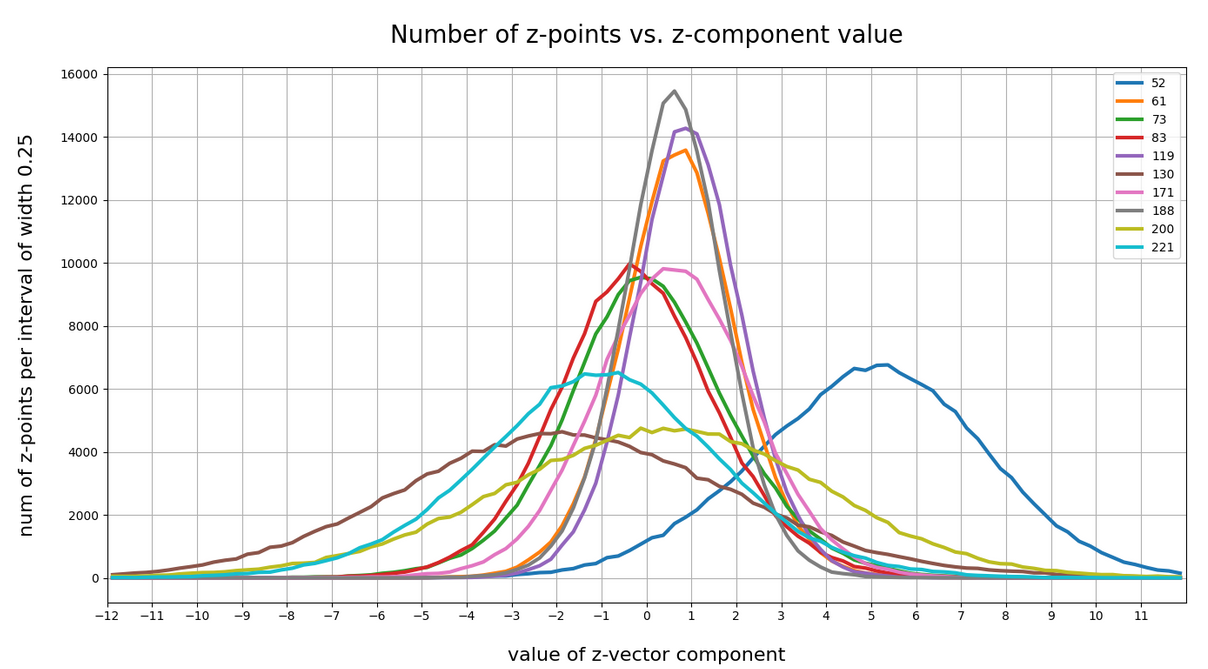
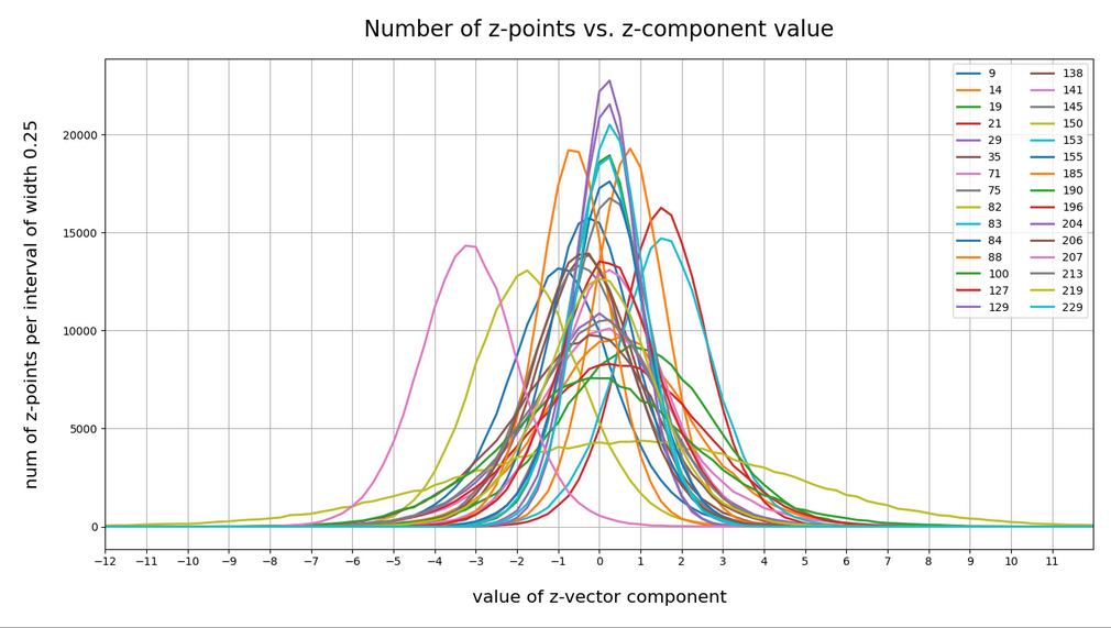
Let me remind you about the shapes of the number distribution for our concrete z-vector components resulting for for CelebA face images. The first plot shows the number densities on sampling intervals of width 0.25 for selected vector components resulting for case I of our experiments. The second plot shows the number densities for the values of selected components of case II.
Ok, these curves do resemble Gaussians and some fluctuations are normal. But can we prove the Gaussian properties of the curves a bit better?
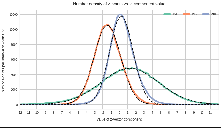
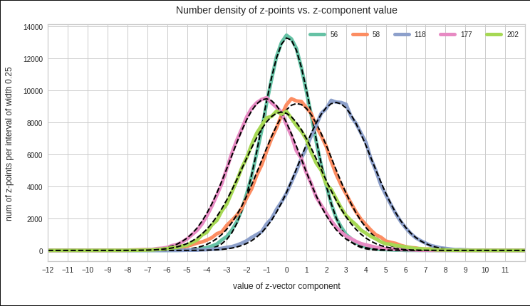
Well, for case II I have drawn the best fits by Gaussian functions with the help of SciPy’s optimize.curve_fit() for 3 and yet another 4 selected components of the latent vectors and the respective number distribution curves. The dashed lines show the approximations by Gaussian functions:
The selected components are part of the list of around 20 dominant component distributions – due to their relatively large standard deviations. But the Gaussian form is consistently found for all components (with some small deviations regarding the symmetry of the curves).
So all in all it looks like as if our convolutional AE has indeed created a multivariate normal z-point distribution in the latent space. As said: This does not exclude correlations …
Pairwise linear correlations of the (normal) probability distributions for the latent vector components?
Now we are a bit bold – and assume the best case for us: Could the approxiate Gaussians distributions for the component values be pair-wise and linearly correlated? What would be a clear indication of a pair-wise linear correlation of our component distributions?
Well, we should find an elliptic form of contour lines in the 2-dimensional distribution for the component pair in the respective coordinate plane of the basic orthogonal LS coordinate system. This imposes quite strong symmetry conditions on the contour lines. The ellipses can be shifted and rotated – but they should remain being ellipses. If non-linear contributions to the correlation had a significant impact this would not be the case.
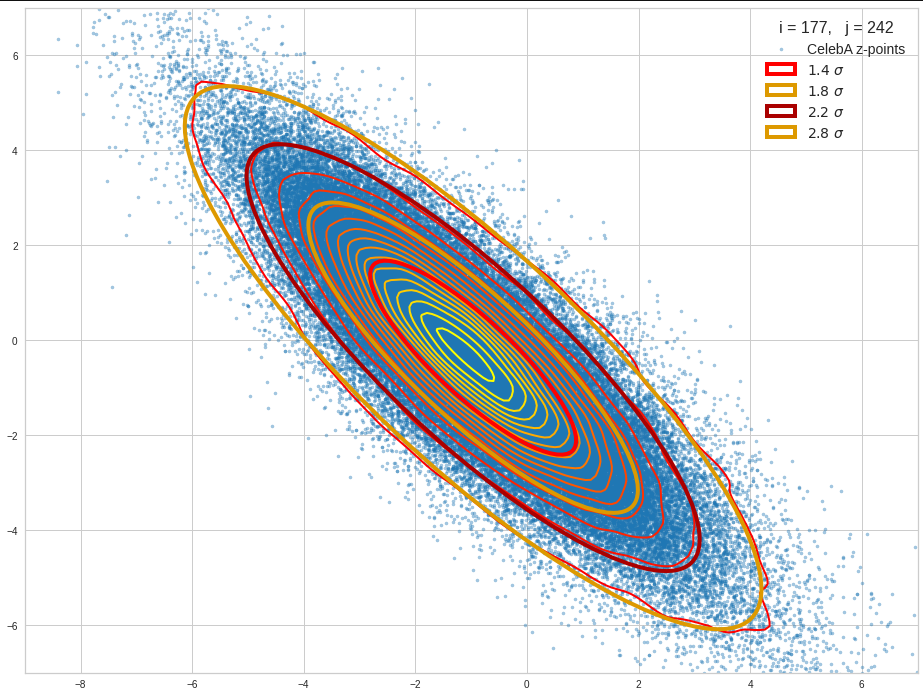
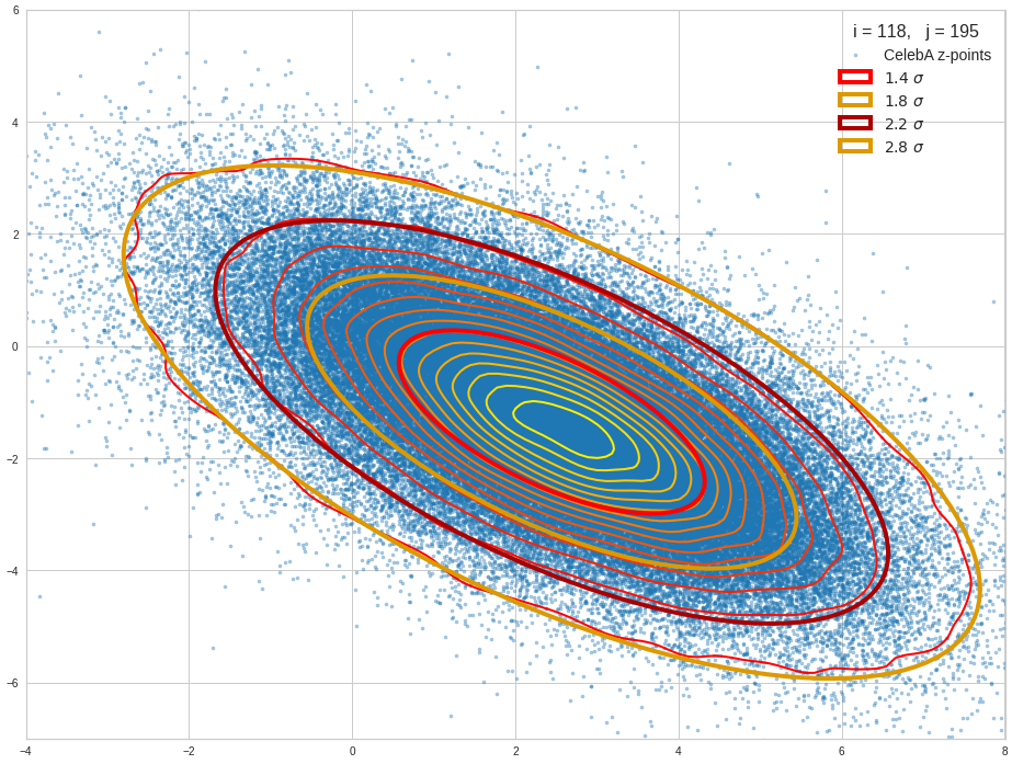
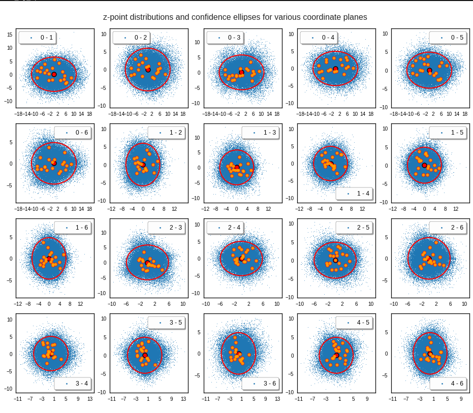
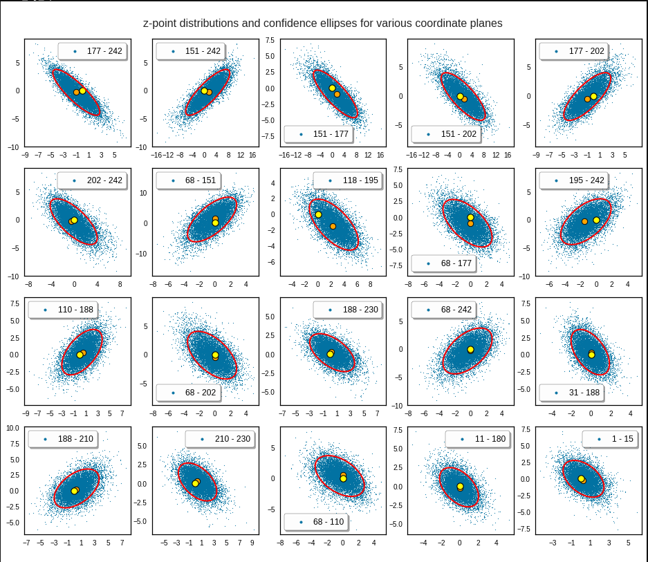
Practically it is not trivial to prove that we have approximately rotated ellipses in 2 dimensions. Satter plos alone do not help: Ellipses fit a lot of plotted distributions of discrete data points quite well. We really need to count number densities to get reliable contour lines. The following plots show such contour lines based on number sampling in rectangles and local smoothing operations with the help of scipy.stats.gaussian_kde().
The fat red and dark orange lines show corresponding confidence ellipses derived from the original CelebA distribution. See below for some remarks on confidence ellipses.
The contours are basically of elliptic shape although they do not show the complete symmetry expected for pure and linearly dependent Gaussian distributions. But overall the confidence ellipses fit quite well into the general form and orientation of the distributions. We also see that for higher σ-levels the coincidence with nearby contours is quite good. The wiggles in the contour change with the z-vector selection a bit.
We conclude that our basic impression regarding an elliptic shape of the z-point distributions is basically consistent with only linearly correlated Gaussian probability density distributions for the component values of the latent vectors.
Approximation of the core of the multivariate z-point distribution by confidence ellipses for component pairs
Above I referred to the boundary of a core of the probability density for two selected vector components. But how would we define the “boundary” of a continuous distribution in the coordinate planes? Answer: As we like – but based on the decline of the approximate Gaussian curves.
We can e.g. pick two times the half-width in each direction or we can use contours defined by confidence levels.
For 2 ≤ fact * σ ≤ 3 we saw already that the contour lines could well be fitted by confidence ellipses. A 3-sigma level covers around 97% of all data points or more. A 2 sigma-level ellipse encircles between 70% and 90% of all data points, depending on the eccentricity of the ellipse. Note that the numbers are smaller for ellipses than for rectangles. I.e. the standard 68-95-99.7 rule does not apply.
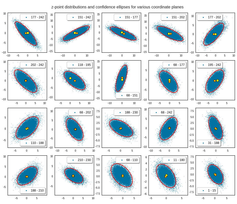
The plots below give you an impression of how well ellipses for a 2σ-confidence level approximate the core of the CelebA distribution in selected 2D coordinate planes of the latent space:
Each of the sub-plots was based on 10,000 statistically selected vectors of the 170,000 available in my test runs. This is a relative low number. Therefore, for a certain diameter of the points in the scatter plot only the inner core appears to be densely populated. The next plots shows the results for a 3 σ-level of the ellipse – but this time for 50,000 vectors. With more vectors we could visually fill the outer regions of the core.
The orange points mark the center of the multidimensional distributions derived from the one-dimensional distribution curves for the components. We see that it does not always appear to be optimally centered. There are multiple reasons: Our functions are not fully symmetric as ideal Gaussians. And equally important: The accuracy of the position depends on the sampling resolution which was coarse. Outliers of the distribution do have an impact.
And how would we explain the appearance of Gaussians and ellipses?
This all looks quite good, despite some notable deviations regarding symmetry and maxima. Gaussians fit at least most of the important probability density curves very well, though not by a 100%. The appearance of an elliptic shape of the inner core of the distribution and the appearance of overall elliptic contour curves can be explained by linear correlations of the Gaussian distributions for the components.
The appearance of normal distributions per component and basically linear correlations is something that really should be explained. I mean, dwell a bit on what we have found:
A convolutional Autoencoder network with more than 10 million adjustable parameters encoded information about human face images in the form of a roughly multivariate normal distribution of z-points in its latent space – with basically linear correlations between the Gaussian curves describing the probability densities functions for the component values of the z-vectors.
I find this astonishing and not at all self-evident. It is one of the most simple solutions for a multidimensional situation one can imagine. The following questions automatically came to my mind:
Does such a result only appear for training images of defined objects with some Gaussian variation in their features? Are the normal distributions a reflection of variations of relevant features in the original data?
Is this a typical result for (convolutional) AEs? How does it depend on the dimensionality of the latent space? Does it automatically come with a large number of z-space dimensions? Is it an efficient way to encode feature differences in the latent space, which (convolutional) AEs in general tend to use due to their structure?
Do I personally have a convincing explanation? No. Especially not, as the data shown above stem from convolutional neural networks [CNNs] without any batch-normalization layers.
A first idea would be that the dominant features of a human face themselves show variations described by Gaussian normal distributions already in the original data and that convolutional filtering does not destroy such distributions during optimization. A problem of this idea lies in the (non-) linear activation functions used at the nodes of the neural maps. Though ReLU, Leaky ReLU and SeLU contain linear parts.
The other problem is the linear form of the correlations. This is a rather simple kind of correlations. But why should an AE choose this simple form into its mapping of image information to latent space vectors after training?
How to generate statistical vectors for the creation of human face images?
The positive message which comes with the above results is that our problem of how to create proper statistical z-vectors decomposes into a sequence of two-dimensional problems. We can use the data of the ellipses appearing in the density-distributions for pairs of vector components to confine the components of statistically generated z-vectors to the relevant region in the latent space. All ellipses together restrict the component values in a well defined form. In the next post I will shortly outline some methods of how we can use the information contained in the ellipses with available algorithms.
Conclusion
In this post we have seen that for the case of a convolutional Autoencoder trained on CelebA human face images the latent vector distributions showed some remarkable properties:
The probability density functions for all component values can roughly be approximated by Gaussian functions. The components appear to be pairwise linearly correlated – at least to first order analysis. This automatically implies elliptic contour curves for the pairwise number density functions of coordinate values. Such contour curves were indeed found with first order accuracy. The core of the probability density for the z-points in the latent space could therefore be approximated by confidence ellipses for a σ-level above σ = 2.5.
The elliptic conditions correspond to a multivariate normal distribution with linear correlations of the variables.
Before we get to enthusiastic about these findings we should be careful and await a further test. All statements refer to a first order approximations. A real multivariate normal distribution would decompose into un-correlated Gaussians and 2D-ellipses of probability densities of component pairs after a PCA transformation.
I shall present the results of a PCA analysis. In later posts I will introduce a related method to restrict the components of statistical vectors to the relevant region in the latent space of our Autoencoder.
Regarding the intimate relation between the ellipses’ main axes to normalized Pearson correlation coefficients I also refer to https://carstenschelp.github.io/ 2018/09/14/ Plot_ Confidence_ Ellipse_ 001.html
I am very grateful that the author Carsten Schelp saved me a lot of time when trying to find a way to program a solution for confidence ellipses. Thank you, Mr. Schelp for the great work.