KMeans as a classifier for the WIFI and MNIST datasets – III – KMeans as a classifier for the WIFI-example

Posted on 25. March 2022 by eremo

In the previous articles of this series

KMeans as a classifier for the WIFI and MNIST datasets – I – Cluster analysis of the WIFI example
KMeans as a classifier for the WIFI and MNIST datasets – II – PCA in combination with KMeans for the WIFI-example

I applied KMeans to the “WIFI” dataset – a small and rather simple training set of the UCI Irvine. The 7 dimensional feature space for this example is defined by the strength of seven different WLAN-signals. The data samples are labeled by numbers specifying four different rooms. We just have 2000 samples. But “simple” does not mean that one cannot learn something of it.

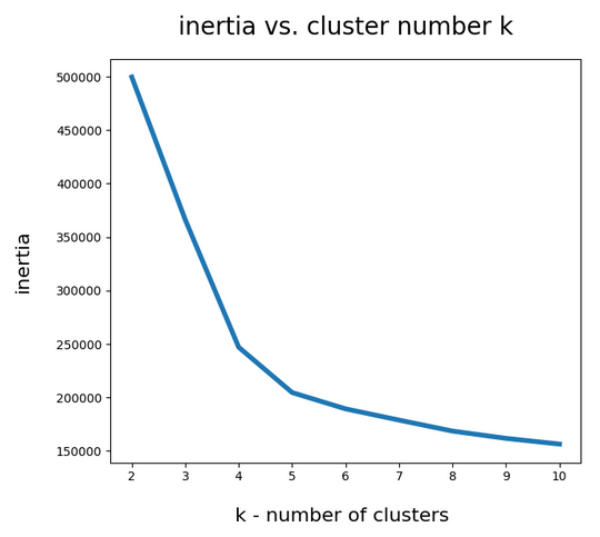
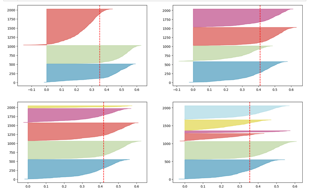
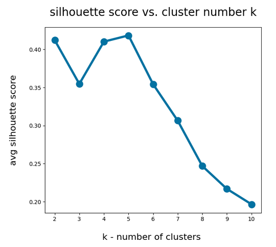
An elbow and a silhouette analysis indicated that the data can well be described by 4 to 5 clusters.
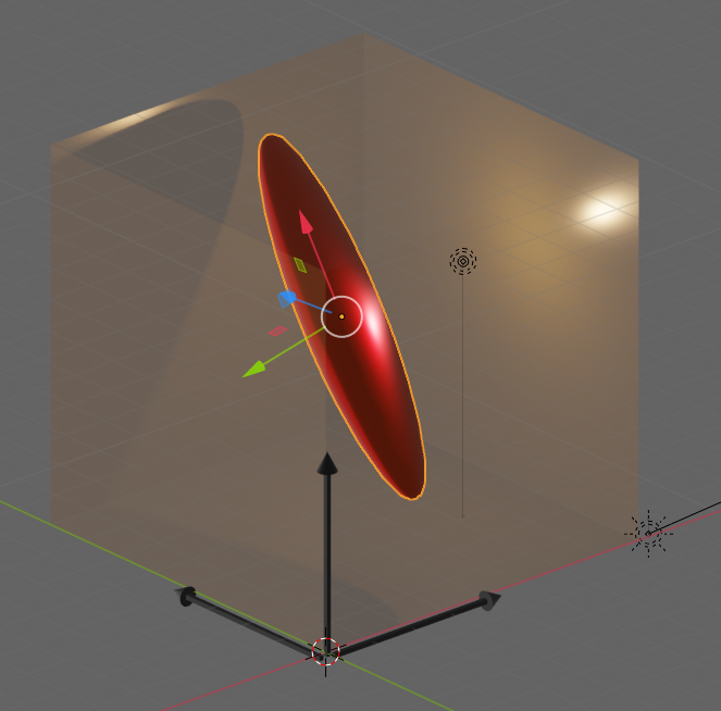
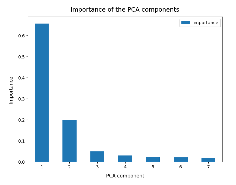
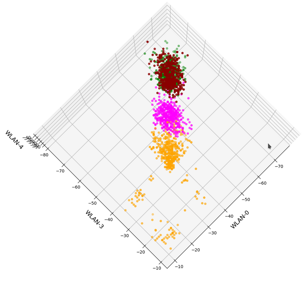
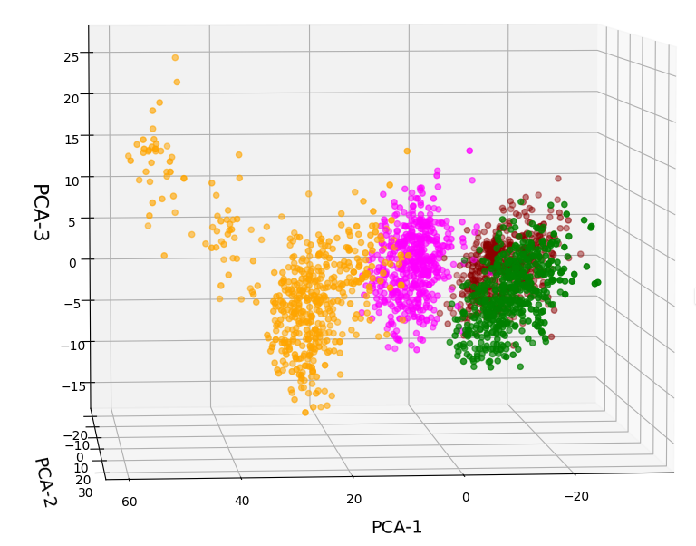
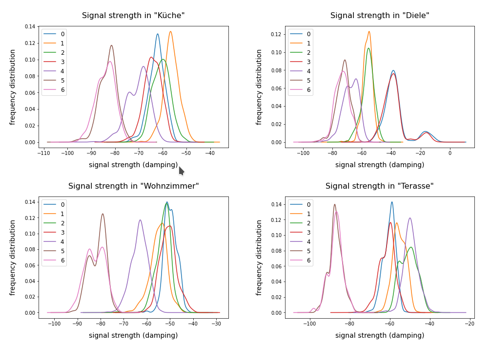
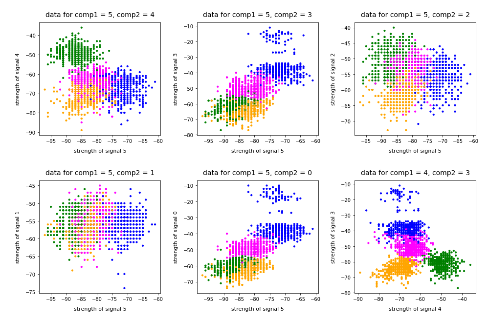
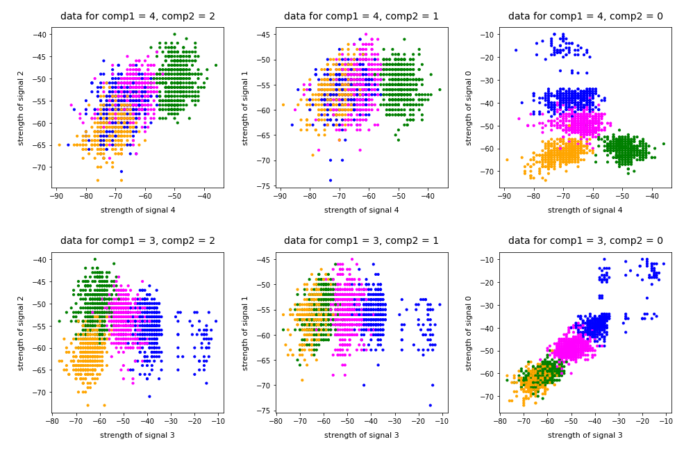
A detailed PCA analysis helped us to understand that the data could basically be described by two primary components whose axes were defined by a diagonal in a two-dimensional sub-space of the original feature space (defined by the features “WLAN-0” and “WLAN-3”) plus an orthogonal axis (defined by “WLAN-4”). As the data points segregated into well separated clusters in the coordinate system of the primary components we could expect that they also segregate well when projected onto two 2-dim sub-spaces of the feature space defined by the signal combinations {WLAN-0/WLAN-4} and {WLAN-3/WLAN-4}.

So we projected the results of a KMeans analysis into a 2-dim sub-space of the 7-dim feature space spanned by two selected “features” (WLAN signals WLAN-0 and WLAN-4). And indeed: For 2 special signal- or feature-combinations we saw a field with 4 to 5 well separated clusters.

As we have well separated clusters – either in sub-planes of the feature space or the space defined by the dominant two PCA components – a legitimate question is: Can we use the cluster information for classifying?

Clusters and classification

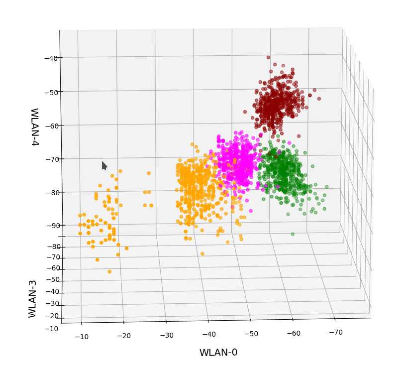
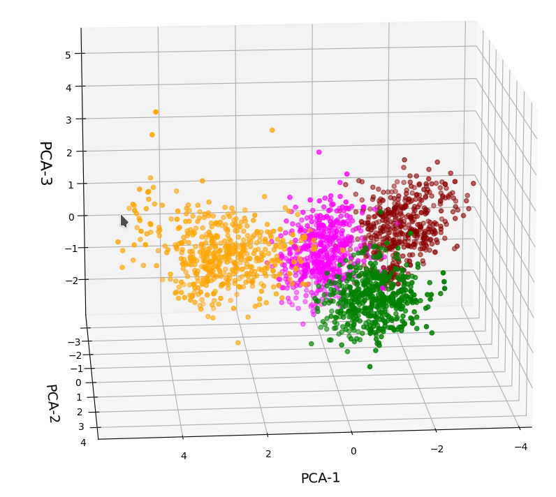
In the special example of the WIFI data the data points can obviously be divided into different “groups” filled by data points which belong to a certain “label” or class (in the WIFI case: a room):

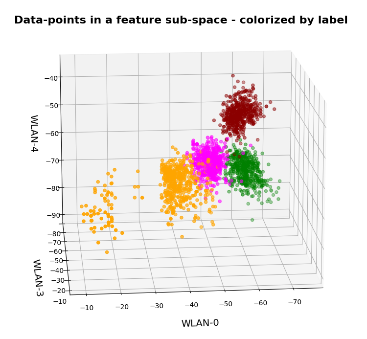
In the plots above the colorization of the data points is given by their label in the plot above. However:
Does this mean that these spatially separated “groups” coincide with the clusters detected by KMeans?

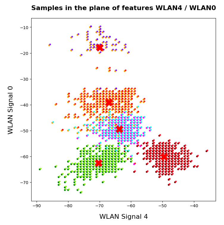
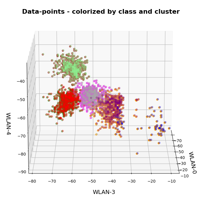
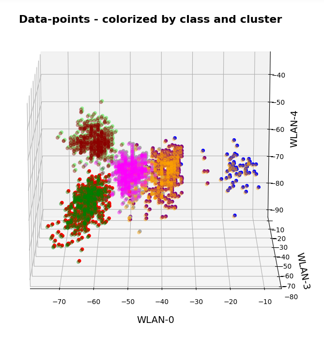
In the next plots I superimposed the data points – first colorized by class and then by cluster with different colors and a slight spatial deviation.

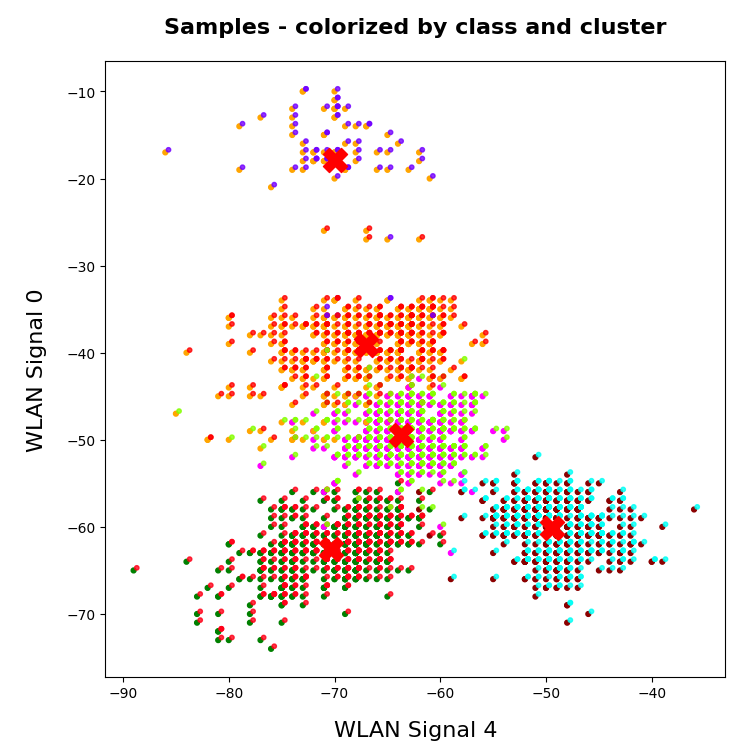
We see that the border of the class related points on average overlaps well with the border of the clusters. Only a few points show a major deviation.

Is this always the case? Of course not!

We see this already when we we just use 2 clusters and colorize the data points according to cluster membership in one of the two clusters:

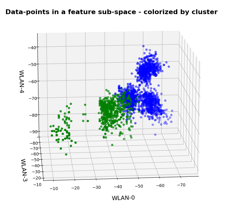
Oops, all the beauty is gone! Members of the previously visual dark-red, green and pink “clusters” would now certainly be members of the first defined “green” cluster. And members of the visual pink and orange clusters would now be members of the “defined” blue cluster. So: Labels may but do strong>not always define clusters.

An important thing we learned by this consideration is that we should at least use a number of cluster greater or equal the number of labels.

But even then the separation may not work. Let us imagine three rooms: In room “A” we only have male persons, in room “B” only female persons and in the third room “C” female persons on one side of the room and male persons on the other – like in some old fashioned dancing courses. If we used the persons’ coordinates to define features and the “male”/”female” attributes as labels and tried a cluster analysis in the feature space we would clearly identify three clusters. However, in the cluster for room “C” we would find a mixture of samples with different labels. Spatial vicinity in the feature space does not mean class identity and a label does not necessarily mean a big distance in the feature space.

Hyperplanes and clusters

The only thing you can hope for with respect to a solvable ML problem is that the data points for different labels may be distributed such that a complicated and curved hyperplane can be found in the multidimensional feature space which separates groups of data points with the same label sufficiently well. But this hyperplane does not necessarily coincide with fictitious borders of some clusters identified by KMeans. We are lucky if the topologically closed surface of a cluster lies completely in a region of the hyperspace separated by complex and topologically open hyperplanes separating data points belonging to one class from other feature space regions which contain data points with different labels.

Not all data ensembles in ML will fall apart in extended clusters each of which dominated by some specific label. Ring like distributions of data samples with identical labels may pose a problem to cluster algorithms – mot only in 2 dimensions.

On the other side: If the labeled data – after some useful transformation – are not well separable in the feature space, then the posed ML task is problematic anyway and the chosen feature definitions may not be appropriate.

Granularity: Hope for label dominance in sufficiently fine grained clusters

What does a label-cluster correlation depend on? Well, if there is an important factor regarding the position of the centroids of KMeans then it is the number of clusters. In the extreme case of as many clusters as data points a super-well defined cluster/label-association exists – but it is not of much use for ML-task. It just represents the most extreme case of overfitting you can think of. It will be useless for new unknown samples.

But the example with the distribution of male/female samples gives you an indication of what we should try: With a growing number of cluster the chances for a fine grained separation into clusters residing on one side of a hyperplane separating samples of different labels rises and with it the chance for a clearer dominance of one label per cluster. This is even true for ring like data distributions: With more then 4 clusters we may even describe a ring like data distribution quite well.

Therefore: If the sample distribution has some reasonable separation hyperplane at all there is a chance that you may find a number of clusters for which each cluster is dominated by a specific label.

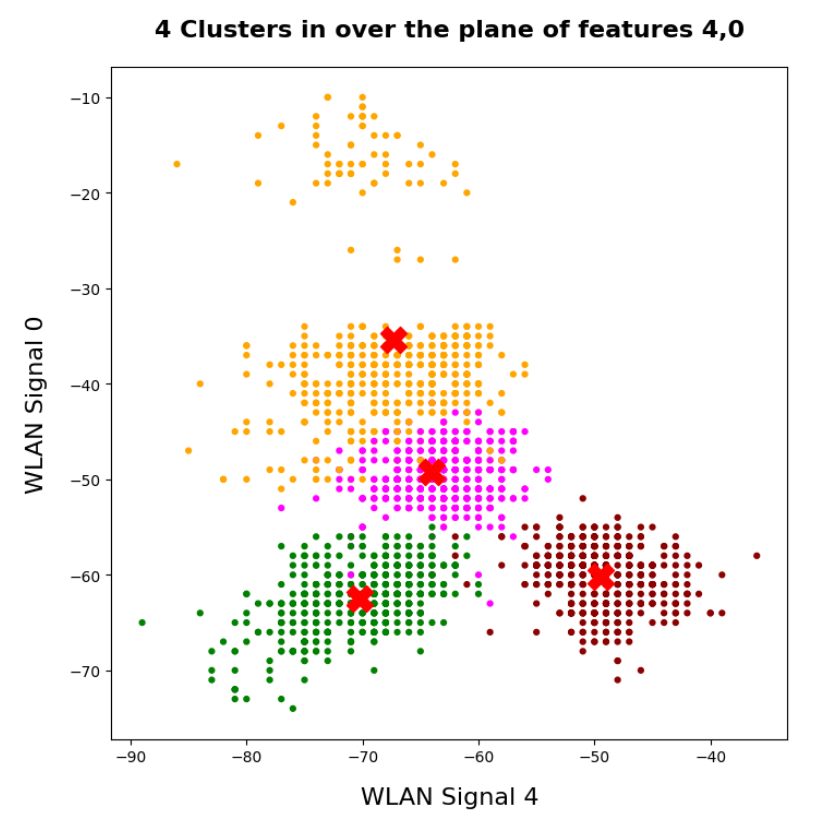
In the case of the WIFI example this is pretty obvious. The following first plot shows the data points colorized according to their labels:

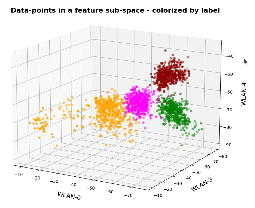
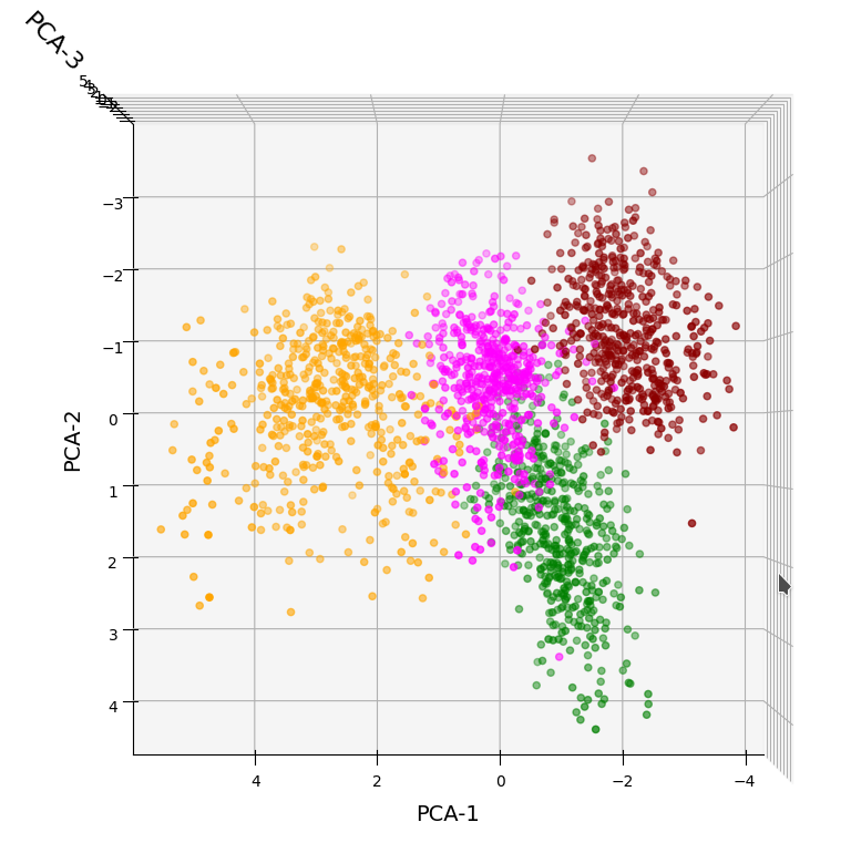
The next plot shows four cluster – with data points colorized according to their cluster membership:

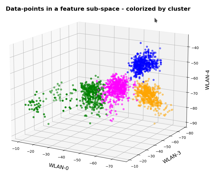
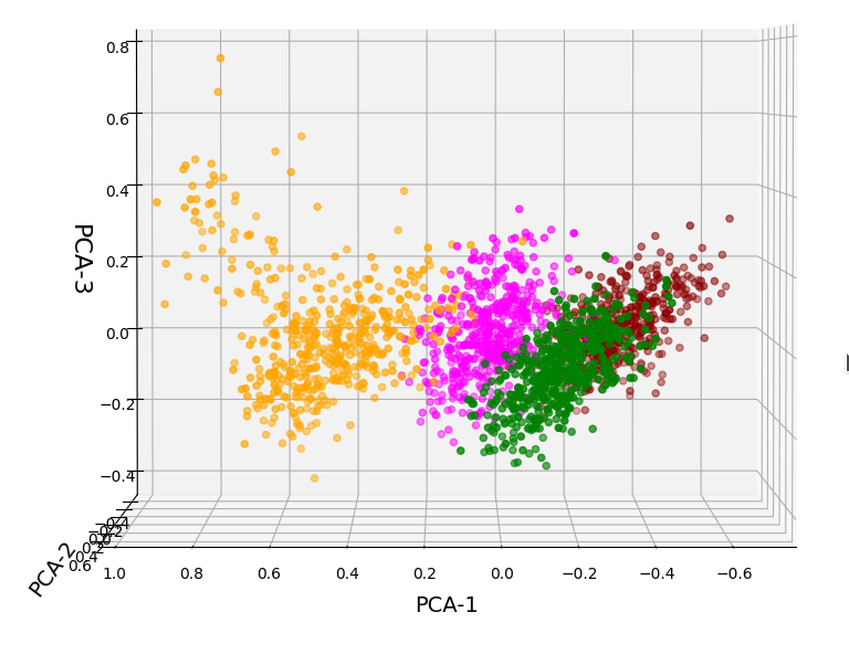
The colors are different (we have no control of it) – but the different data point “clouds” in the pictures coincide rather well. Only some data points do not behave well. We can again use the trick we iused in 2 dimensions and superimpose data points with colorization according to cluster and class:

How do we define a classifier by the help of KMeans?

We need a predict()-function which predicts a label from a predicted cluster membership. The recipe is rather simple:

Define the number of cluster you want to use.

Use KMeans for a cluster analysis of a training set of samples.
Predict the cluster-membership of a sample with the help of the fitted kmeans-object and its predict()-function.
Get the labels of the samples belonging to a specific cluster.
Find out what the amount of samples with a certain label for a cluster is and compared the data.
Find the label which contributes most samples to a cluster. Check the relative amount of deviating data points with other labels. Should be sufficiently small…
Build a dictionary which associates the cluster number with its dominant label.
Build a prediction function for yet unknown data points. It first predicts the cluster and then the associated label.

You should then test the accuracy of your new cluster-based classifier model on test data.

More clusters than labels?

What will happen to such an algorithm if you use more clusters than labels? Short answer: Nothing – as long as each cluster is really dominated by a specific label. More precisely: A vast majority of your clusters should exhibit contributions from data points with one specific label to an amount significantly far beyond the statistical average. Having more clusters means that under reasonable conditions we just have more than one cluster predicting a certain label. For the case of the WIFI example this means that we can work with five clusters without getting nervous.

Application to the WIFI example

As the clusters represent the labels quite well we expect very good values for the recall values. The experiment is pretty simple. I just present the resulting confusion matrices for the four labels (identifying rooms) and different numbers of clusters “nclus”. I first show you a presentation with seaborn, which explains, how to interpret rows and columns:

nclus = 5

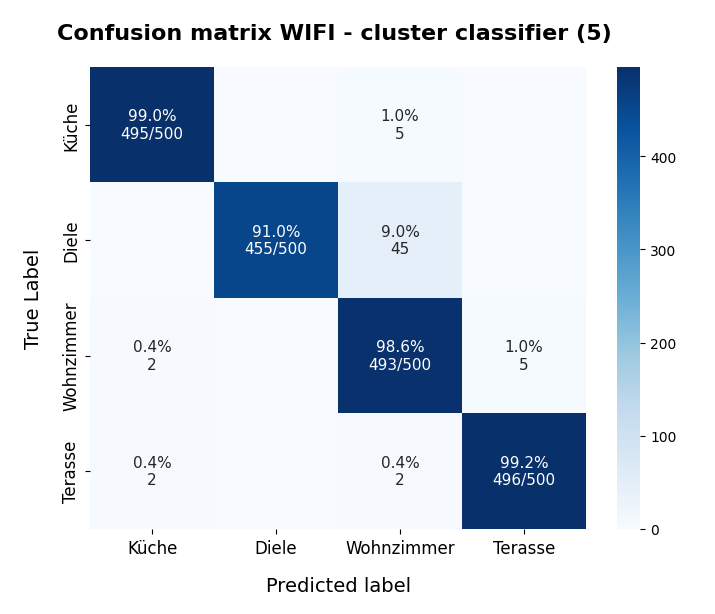
Here I used five (5) clusters and included all samples in the calculation. I.e. I did not separate a training set from a test set of data points.

Confusion matrices for different numbers of clusters

nclus = 4

[[496   0   4   0]
 [  0 425  75   0]
 [  2   0 492   6]
 [  2   0   2 496]]
num of wrongly predicted samples:  91  :: avg_err =  0.0455

The “avg_err” gives you the number of wrongly predicted samples divided by the total number of samples. We see that 4 clusters have a problem with the differentiation of the data points for the room “Diele”.

nclus = 5

[[495   0   5   0]
 [  0 455  45   0]
 [  2   0 493   5]
 [  2   0   2 496]]
num of wrongly predicted samples:  61  :: avg_err =  0.0305

nclus = 6

[[499   0   1   0]
 [  0 452  48   0]
 [  5   0 490   5]
 [  2   0   2 496]]
num of wrongly predicted samples:  63  :: avg_err =  0.0315

nclus = 7

[[499   0   1   0]
 [  0 492   8   0]
 [  4  38 455   3]
 [  2   0   3 495]]
 num of wrongly predicted samples:  59  :: avg_err =  0.0295

nclus =

num wrongly predicted samples:  58  :: avg_err =  0.029

nclus = 9

[[499   0   1   0]
 [  0 484  16   0]
 [  4  16 476   4]
 [  2   0   2 496]]
num of wrongly predicted samples:  45  :: avg_err =  0.0225

All data above were derived for the same random_state-variable to KMeans.

However, this result depends on the initial shuffling of the samples, the random_state parameter and the initial statistical distribution of the centroids by KMeans. And other hyperparameters … The next plot shows a slightly different result for nclus = 9:

nclus = 9

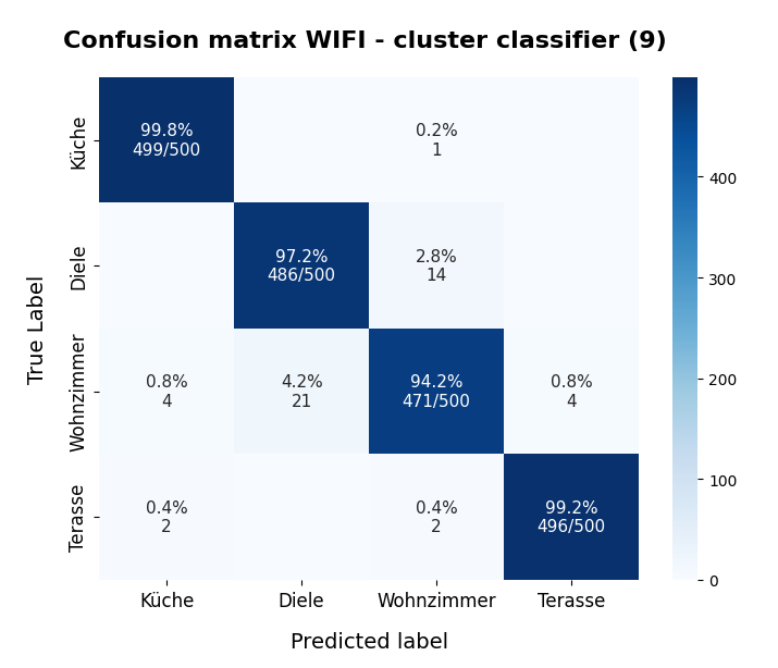
This means: Nine cluster give us a reasonably fine grained resolution in the case of the WIFI example.

But: Note that the problem areas in the confusion matrix have changed. “Diele” is handled a bit better, but “Wohnzimmer” is not so sharply separated as before. This is not astonishing as we saw a significant mix of data of different labels for different clusters above already:

After nclus = 9 we do not get much better – and dance around an average error of 0.025 => 2.5%:

nclus = 10

num of wrongly predicted samples:  55  :: avg_err =  0.0275

nclus = 11

num of wrongly predicted samples:  52  :: avg_err =  0.026

nclus = 25

num of wrongly predicted samples:  40  :: avg_err =  0.02

Being conservative we can say that our simple cluster based classifier approaches an accuracy around 97.4%. Not so bad regarding the crudeness of our approach! A random forest algorithm reaches something above 98.2%. This is not so much better.

Results after a separation of test data samples

I divided the data set than into 1500 train and 500 test samples.

For 9 clusters I got:

nclus = 9

[[374   0   1   0]
 [  0 362  13   0]
 [  3  17 352   3]
 [  2   0   2 371]]
num wrongly predicted train samples:  41  :: avg_err =  0.027333333333333334
num wrongly predicted train samples:  8  :: avg_err =  0.016

But these numbers depend strongly on the splitting – even if we split stratified. Another run gives:

nclus = 9

[[374   0   1   0]
 [  0 352  23   0]
 [  3   0 369   3]
 [  1   0   2 372]]
num wrongly predicted train samples:  33  :: avg_err =  0.022 
num wrongly predicted test samples:  11  :: avg_err =  0.022

Other runs may even give higher average error values. The variation depend upon of how many critical data points in the intermixing zone were omitted in the train samples. At least the results are not too different from the ones named above.

Conclusion

In this article I presented a very simple method by which a cluster algorithm can be used as a classifier. When we applied the approach to the rather simple WIFI example we saw that this worked pretty well.

What we in addition should try is to combine the classifier with a dimension reduction based on a PCA-analysis. From the results of a previous post we would expect that a cluster classifier should work well on the WIFI data after a transformation and projection of the samples’ data points into a 3-dimensional space spanned by the most important orthogonal main component axes. This is the topic of the next post in this series:

KMeans as a classifier for the WIFI and MNIST datasets – IV – KMeans on PCA transformed data

Ceterum censeo: The worst fascist today who must be denazified is the Putler.

KMeans as a classifier for the WIFI and MNIST datasets – II – PCA in combination with KMeans for the WIFI-example

Posted on 14. March 2022 by eremo

I continue with my series of posts about using KMeans as a classifier for some simple ML datasets. In the last post

KMeans as a classifier for the WIFI and MNIST datasets – I – Cluster analysis of the WIFI example

I applied KMeans to the “WIFI” dataset which was discussed in the German “Linux Magazin”; see the Nov and Dec editions of 2021. We found 4 to 5 well separated clusters in a projection of the data points onto a 2-dimensional space defined by just two out of seven features.

I briefly discuss how this result is related to a PCA analysis. In my opinion the discussion in the “Linux Magazin” was a bit misleading regarding this point.

PCA analysis

A PCA analysis helps to identify the main orthogonal axes of the distribution of the samples’ data-points in their multidimensional “feature space”. If the data points for the samples are distributed in all directions and over all regions of the feature space in a similar way we may indeed need all of the feature spaces’s dimensions to describe the data distribution. Still, we could find some complicated curved hyperplanes which separate groups of data points with identical label quite well.

But often the data points are positioned along certain preferred directions, i.e. the data points are located along specific lines or (multidimensional) flat planes in the feature space – not withstanding an additional clustering. In such cases the data distribution may exhibit some intrinsic major axes in the feature space AND/OR the distribution may be confined to a subspace of the original feature space. The sub-space is defined and spanned by fewer axes than the original space. We speak of the “primary components” of the data distribution when we refer to the (orthogonal) axes of such a sub-space.

Of course, we can span the full original feature space by the most important primary component axes plus some extra orthogonal axes. I.e., we just need the same number of main components as the dimension of the original feature space. Then we get a new coordinate system which describes the vector space of the original features in a different way: The differences are

another orientation of the main component axes in comparison with the original axes,
a difference in the position of the origins of the two coordinate systems.

Of course, there is a mathematically well defined transformation which maps coordinates of data points with respect to the original feature spaces axes to coordinates in a coordinate system defined by the main component axes.

Of course, we can project a vector describing a data point onto unit vectors along the axes of either coordinate system. By using these special components we can describe the data distribution in terms of a sub-space spanned by only the most important primary component axes. A projection of ML data points to primary component axes is equivalent to a reduction of the dimensionality of the ML problem. Whenever we find that we can use fewer main component axes than the feature space’s number of dimensions to describe the data distribution reasonably well we can reduce the dimensionality of the problem: We project the original data vectors in the feature space to the axes of the main components’ coordinate system with fewer dimensions than the feature space.

How do we measure the “importance” of a main or primary component?

A metric for the importance of a primary component axis is its contribution to the so called “explained variance”. This quantity measures correlations of data in the original feature space and thus also the amount of information residing in the data.

From a mathematical point of view determining the main component axes corresponds to the diagonalization of the so called covariance matrix and the identification of eigenvectors. (You can find a short explanation in the books of S. Rashka on “Python Machine Learning”, 2016, PACKT or the book of J. Frochte on “Maschinelles Lernen”, 2019, Carl Hanser.) The eigenvectors define the directions of the main components’ axes. The variation of the data along such a main component axis contributes to the total variance by its measure of specific correlations, i.d. weighted quadratic data point distances. We are interested in finding those main component axes for which the projected data distribution explains most of the data variation.

Note that the axes which a PCA-analysis determines are orthogonal axes. Thus PCA describes a transformation of vectors in the feature space from one coordinate system with orthogonal axes to another coordinate system with orthogonal axes. Geometrically, this can be described by a sequence of a translation, followed by a rotation – and in case of a dimensionality reduction in addition by a projection.

Let us visualize an example. The following picture shows the surface of an asymmetric “ellipsoidal” data distribution in a 3-dim feature space. (Actually, the image does not display a real ellipsoid – but we ignore the differences for reasons of simplicity.) The dark arrows in the picture indicate the orthogonal axes and unit-vectors per dimension of the 3-dim feature space. The colored arrows of the ellipsoid show the direction of the main component axes of the “ellipsoid”.

Regarding the dimensions of the ellipsoid the elongation along the red vector is biggest. The width of the data point distribution in the direction of the blue vector is significantly smaller, but still bigger than in the direction of the green vector. So, we would expect that the two main component axes in the directions of the red and the blue arrows explain most of the data variation in the feature space. The projections of the data point vectors in a coordinate system defined by the main component axes onto the “green” axis would only give us rather small values. Therefore, we can reduce the dimensionality of the problem by describing the data distribution in only two dimensions: We project the vectors of the original data points in the feature space onto the two most important main component axes – in the directions of the red and the blue unit vectors.

Note: The axis in the direction of the dominant elongation of the ellipsoid has a diagonal orientation in the feature space. This means that all of the three original features contribute to the data points’ distribution in this direction. Therefore, the following point must be underlined:

A PCA analysis is not a selection process with respect to the original features. A vector describing a main component axis of the data distribution is a
linear combination of all unit vectors along various original axes of the feature-space. Normally many – if not all – original features contribute to a main component axis.. Without a detailed analysis you can not assume that only one or two original features determine the primary component axis.

In particular: You cannot assume that only one special feature dominates a main component axis. Unfortunately, the text in the Linux Magazin on the WIFI example could be read and interpreted in this way. So, let us have a closer look at the reason, why the projections of the WIFI-data from the original 7-dimensional feature-space onto a reduced 2-dim space of the signal-combinations [WLAN-4, WLAN-0] or [WLAN-3, WLAN-0] worked so well.

How many main components dominate the variance of the WIFI data distribution?

How many main components explain most of the variation of the samples’ data of the WIFI example? How do we get the required information about the contribution to the explained variance from PCA applications? Sklearn’s PCA implementation provides the usual “fit()”-function to perform the PCA calculation for a given data set. But it also provides an array named “explained_variance_” which contains the individual contributions of the main components to the “explained variance“.

So, as a first step, we simply try and apply Sklearn’s PCA()-function directly to the original WIFI data given in their 7-dimensional feature space. I.e. without any scaling. Just as it was done in the Linux Magazin. The bar plot below displays the “importance” of a maximum of 7 main components. The importance of each component is measured by its normalized contribution to the “explained variance”:

An accumulation gives the following percentages:

We see that only two of the main PCA components already explain 85% of the data variance in the feature space. We thus could choose these two main components as our “primary” components. But this does NOT automatically mean that only two features dominate the data distribution in the feature space.

Which features determine the primary components’ orientation?

As we have discussed above the projection of a unit vector along the main component axis onto the original axes of the feature-space may give similarly big values for each of the features. It is rather seldom that only a few features determine the direction of a main component’s axis.

But: The WIFI data are (on purpose?) indeed distributed in a very special way. Actually, only two original features determine the direction of the most important primary component’s axis already quite well. And just one feature dominates the second most important PCA component. So, in the WIFI example the first and the second main components are oriented more or less within a 2-dim feature plane and along a special feature axis, respectively. I.e. the data are more or less confined to a 3-dimensional sub-space of the feature space. How and where from did I get this information?

Sklearn’s function “PCA()” returns a reference to an object, which after a call to its method “fit()” has a filled property “components_“. This array gives us the 7 vector-components of each unit vector oriented along a PCA main component axis with respect to the various original axes of the feature space. I.e. we get the components of unit vectors along main component axes in terms of the original coordinate system spanning our feature space. The related coefficients of the vector tell us whether the main component axes are confined to a subspace spanned by just a few original features.

Below, the elements (rows) of the array were reversely sorted by the the contribution of the main component to the “explained variance”. So the first two rows correspond to the two most important PCA main components.

[6.22e-01 7.47e-04 1.03e-02 6.29e-01 2.02e-01 3.03e-01 2.91e-01]
 [1.71e-01 9.05e-02 4.31e-01 1.95e-01 8.50e-01 1.02e-01 7.62e-02]
 [2.41e-01 2.78e-01 2.18e-01 2.90e-01 9.80e-02 5.28e-01 6.67e-01]
 [1.67e-01 3.44e-01 7.05e-01 1.69e-01 4.22e-01 9.65e-02 3.75e-01]
 [1.13e-01 1.77e-01 3.15e-01 1.33e-01 1.82e-01 6.97e-01 5.66e-01]
 [6.37e-01 2.31e-01 3.28e-01 6.45e-01 1.26e-01 1.32e-02 3.22e-02]
 [2.80e-01 8.43e-01 2.50e-01 1.42e-01 2.43e-02 3.52e-01 5.12e-02]]

The first primary component has vector-components along the original axes of the feature space given by

6.22e-01, 7.47e-04, 1.03e-02, 6.29e-01, 2.02e-01, 3.03e-01, 2.91e-01

The features, i.e. the WLAN signals, are numbered in the given order from left to right. Obviously, the features “WLAN-0” and “WLAN-3” dominate the direction of the first primary component.

The second main component

1.71e-01, 9.05e-02, 4.31e-01, 1.95e-01, 8.50e-01, 1.02e-01, 7.62e-02

is instead dominated by he feature “WLAN-4”.

Actually, a closer look shows that the signal “WLAN-6” dominates the third main component by a relatively big value. This might be an indication that we had better used three primary components instead of two … I come back to this point below.

So, what do we learn from the results of the projections of the PCA unit vectors onto the axes of the feature space?

In the very special case of the WIFI example around 3 original features dominate the overall data distribution.
In the WLAN-0/WLAN-3 plane we should see an approximate diagonal distribution of data. Reason: the vector components are of almost equal size.
As we already know from an elbow-analysis we have 4 to 5 clusters. So, we should see them clearly in a 3D-plot for the axes WLAN-0, WLAN-3 und WLAN-4.
If the data are well separated into clusters along the diagonal in the WLAN-0/WLAN-3 plane AND the WLAN-4 direction then they will also be well separated in the 2-dim space of the 2 main PCA components.

Ok, let us visualize it. The next plot shows the data distribution from a view almost perpendicular to the WLAN-3/WLAN-4 plane. The colors indicate the labels of the data (i.e. the rooms where the strength of each of the 7 WLAN signals has been measured).

3D-plot of the WIFI data distribution in the space of the dominant 3 original features – the WLAN-3/WLAN-4 plane

We already see the clustering. The next plot shows the data distribution from a direction almost perpendicular to the WLAN-0/WLAN-4 plane.

3D-plot of the WIFI data distribution in the space of the dominant 3 original features – the WLAN-0/WLAN-4 plane

And now a view from above showing the diagonal distribution of very many data points. We clearly see that there is something strange going on in the “orange” room.

3D-plot of the WIFI data distribution in the space of the dominant 3 original features – the WLAN-3/WLAN-0 plane

So far, so good! We have again identified the clusters which we already got familiar with in my last post.

Data distribution in the vector space of the three most important PCA components

In full consistency with the results derived above we expect a good cluster separation in the plane of the first two main PCA components. These components are called “PCA-1” and “PCA-2” in the following plot:

3D-plot of the transformed WIFI data distribution in the space of the dominant 3 PCA components – the PCA-1/PCA-2 plane

But looking from a different perspective, we see that there still is a significant distribution along the axis of the third main component – at least with the scaling used along the PCA-3 axis.

3D-plot of the transformed WIFI data distribution in the space of the dominant 3 PCA components – the PCA-1/PCA-3 plane

Even when we take into account the different scales of the axes: The spread in z-direction (PCA-3) is relatively big compared with the data spread in the PCA-2 direction. Again, we see that the data indicate three main components. Why did we not get this information already in our bar plot for the “explained variance”?

Working on scaled data

Well, part of the answer to the last question is that we did not really treat the various WLAN signals equally well. Actually, for very simple reasons, a PCA analysis of really independent features with different measurement units should be applied to scaled data. So, just for curiosity’s sake, let us apply Sklearn’s StandardScaler() to our WIFI data ahead of a PCA-analysis. Then, we indeed get a different bar plot:

The elbow is now centered at a point corresponding to 3 main components! Below I show respective 3D-plots for the standardized and PCA-transformed data:

3D-plot of the scaled WIFI data distribution in the space of the dominant 3 PCA components – the PCA-1/PCA-3 plane

3D-plot of the scaled WIFI data distribution in the space of the dominant 3 PCA components – the PCA-1/PCA-2 plane

However, the 5th cluster – a subcluster of the orange one – is no longer so clearly visible as before. This is due to the fact that the standard deviation of the data around the mean value of each feature is adjusted to a value of 1.0 with StandardScaler(). A MinMaxScaler() does a better job:

In the case of the WIFI example there is also a strong counter-argument against scaling:
The individual features and their scales are NOT really independent of each other. A weaker signal or a specific spread around the mean value of a specific signal do actually mean something! When we have multiple maxima in a signal distribution (see the previous post) this carries some important information – and then the adjustment of the standard deviation to a standard value is not a really good idea. This means that it depends on the data and their meaning which kind of scaler one should use ahead of a PCA analysis.

Conclusions

The existence of a few primary components does not automatically mean that only a few features contribute to the data distribution’s variance in the features space. However, in the case of the WIFI data example we have a special situation for which only three out of seven features do determine the primary components and the direction of the respective preferred axes of the data distribution. We also saw that we may have to scale feature data properly before applying a PCA analysis.

In the next post of this series

KMeans as a classifier for the WIFI and MNIST datasets – III – KMeans as a classifier for the WIFI-example

we shall answer the question whether and how we can use the cluster algorithm KMeans also as a classifier for the WIFI data.

Ceterum censeo: The worst fascist today who really and urgently must be denazified is the Putler.

KMeans as a classifier for the WIFI and MNIST datasets – I – Cluster analysis of the WIFI example

Posted on 3. March 2022 by eremo

In the November and December 2021 editions of the German “Linux Magazin” R. Pleger discussed a simple but nevertheless interesting example for the application of a cluster algorithm. His test case was based on a dataset of the UCI Irvine. This dataset contains 2000 samples with (fictitious?) data describing WIFI signals which stemmed from seven WLAN spots around a building. The signal strength of each source was measured at varying positions in four different rooms. I call the whole setup the “WIFI example” below.

One objective of the articles in the Linux Magazin was to demonstrate how simple it is today to apply basic Machine Learning methods. In a first step the author used a ML classifier algorithm to determine the location (i.e. the room) of a measuring instrument just from the strengths of the different WIFI signals. This task can be solved by a variety of algorithms – e.g. by a Decision Tree, SVM/SVC or a simple Multilayer Perceptron. The author used Sklearn’s RandomForestTree. This method is a good example for the powerful “Ensemble Learning” technique. When applied to the simple and well structured WIFI example it predicts the rooms for test samples with an accuracy of more than 98%.

The author afterward performed a deeper analysis of the WIFI data via Kmeans, MiniBatchKMeans and PCA. His second article underlined a major question, which sometimes is not taken seriously enough:

Do the data, which we feed into ML algorithms, really cover all aspects of the problem? Is the set of target labels complete or sufficient in the sense that the separation of the samples into labeled groups really reflects the problem’s internal structure? Or do the data contain more information than the labels reveal?

Unfortunately, in my opinion, the Linux Magazine covered an important point, namely the relation of the results of a PCA analysis to a 2-dimensional cluster visualization, in an incomplete and also slightly misleading way. In addition another interesting question was not discussed at all:

Can we use KMeans also as a classifier? How would we do this?

In this series of posts I want to dig a bit deeper into these topics – both for the WIFI example and also for the MNIST dataset. For MNIST we will not be able to visualize clusters as easily as for the WIFI example. Therefore, we should have a clear idea about what we do when we use clusters for classifying.

In this first post I focus on the results of a cluster analysis for the WIFI example. In a second article I will discuss the relation of cluster results to a PCA analysis. A third post will then present a very simple method of how to turn a cluster algorithm into a classifier algorithm. In later articles we shall transfer our knowledge to the MNIST data. More precisely: We shall combine a PCA analysis with a cluster classifier to predict the labels of handwritten digit images. We will use the PCA technique to reduce the dimensions of the MNIST feature space from 784 down to below 80. It will be interesting to see what accuracy we can reach with a relatively crude clustering approach on only about 30 main PCA components. As a side aspect we shall also have a look at standardization and normalization of the MNIST data.

I do not present any code in the first three posts as the required Python programs can be build relatively straight-forward and most of the core statements were already given in the Linux Magazin. You unfortunately have to buy the articles of the magazine; but see https://www.linux-magazin.de/ausgaben/2021/11/maschinenlernen/. However, as soon as we turn to MNIST I shall provide a Jupyter notebook.

The WIFI example: Two thousand samples, each with data for the signal strength of seven WLAN sources measured in four rooms

You can download the data WIFI data set from the following address:
https://archive.ics.uci.edu/ml/machine-learning-databases/00422/wifi_localization.txt

The feature space of this is example is 7-dimensional: 7 WLAN spots provide WIFI signals in the building. We have 2000 samples. Each sample provides the signal strength of each of the WLAN sources measured at different times and positions within a specific room. An integer number in [1,4] is provided as a label which identifies the room. The following plot shows the interpolated frequency distribution over the signal strength for each of the 7 signals in the four rooms:

Cluster analysis of the WIFI data – more than four rooms?

The original label-data of the WIFI example imply the existence of four rooms. But can we trust this information? The measurements in the room, which we called “Diele” in the plots above, indicate a consistent second peak for both the signals 0 and 3. Is this due to an opening into another room?

A simple method to analyze the inner structure of the distribution of data points in a configuration or feature space is a “cluster analysis”. The KMeans algorithm provides such an analysis for an assumed number of clusters.

KMeans is a basic but important ML method which reveals a lot about the data distribution in feature space and indirectly about the complexity of hyperplanes required to separate data according to their labels. Among other things KMeans determines the positions of cluster centers – the so called centroids – by measuring and systematically optimizing distances of samples to assumed centroids. Actually, the sum over all intra-cluster variances, i.e. the summed quadratic distances of the associated samples to their cluster’s centroid, is minimized. The respective quantity is called “inertia” of the cluster distribution. See e.g. the excellent book of P. Wilmott, Machine learning – an applied mathematics introduction” on this topic.

A simple method to find out into how many clusters a distribution probably segregates is to look for an elbow in the variation of the inertia with the number of clusters. When we look at the variation of inertia values with the number of potential clusters “k” for the WIFI example we get the following curve:

This indicates an elbow at k=4,5.

Another method to identify the most probable number of distinct clusters in a multi dimensional data point distribution is the so called “silhouette analysis”. See the book of A. Geron “Hands-On Machine Learning with Scikit-Learn, Keras and Tensorflow”, 2n edition, for a description. For the WIFI example the plots of the silhouette score data support the result of the elbow analysis:

The second plot shows ordered silhouette data for k = 3,4,5,6 clusters. Again, we get the most consistent pictures for k=4 and k=5.

So, the data indicate a fragmentation into 4 or 5 clusters. How can we visualize this with respect to the feature space?

Scatter plots for 2-dim sub-spaces of the feature space

A general problem with the visualization of cluster data for multidimensional data is that we are limited to 2, maximal 3 dimensions. And a projection down to two dimensions may not reflect the real cluster separation in the multidimensional feature space in a realistic way. But sometimes we are lucky.

We shall later see that there are two primary components which dominate the data and signal distributions in the WIFI example. A major question, however, is whether we will also find that only a few original features contribute dominantly to these major components. A PCA analysis does not mean that a “primary component” only depends on the same number of features!

As I did not know the relation of “primary components” to features I just plotted the results of “KMeans” for a variety of 2-dim signal combinations. I used Sklearn’s version of KMeans; due to the very small data ensemble KMeans is applicable without consuming too much CPU time (this will change with MNIST; there we need to invoke MiniBatchKMeans):

Note that the colorization of the data points in all plots was done with respect to the cluster number predicted by KMeans for the samples – and not with respect to their labels.

It is interesting that the projections onto two special feature combinations – namely WLAN-4/WLAN 0 and WLAN-3/WLAN-0 signal – show a very distinct separation of the clusters.

Four or five clusters ?

The data displayed above depend a bit on the initial distribution of cluster centers as an input into the KMeans algorithm. But for 4 and 5 clusters we get very consistent results. The next plots show the positions of the centroids:

This time the colorization was done with respect to the labels. What we see is: Five clusters represent the situation a bit better than only 4 clusters.

When we align this with the rooms: Five “rooms” may describe the signal variation better than only 4 rooms. The reason for this might be that one of the four rooms has a wall which partially separates different areas from another. We often find this in “entrances” [German: “Diele”] to houses. Sketches of the rooms in the Linux Magazin article actually show that this is the case. And, of course, such a wall or an opening into another room would have an impact on the damping of the WLAN signals.

Addendum 19.03.2022: Comparing clusters with groups of labeled data points

An important question which we have not answered yet by the images shown above is the following:

How well do clusters coincide with groups of data points having a specific label?

Note that in general you can not be sure that clusters reflect data points of the same label. Actually, a cluster is only a way to describe a close spatial vicinity of data points in some region of the multidimensional feature space. I.e. some kind of clumping of the data points around some centroids. But spatial vicinity does not necessarily reflect a label: A label border may often separate data points which are very close neighbors. And a cluster may contain a mixture of samples with different labels ….

Well, in the case of the WIFI example the identified 4 to 5 clusters match the groups of data points with different labels quite well. Below I superimposed the sample’s data points with different colors: First I colorized the data points according to their label. On top of the resulting scatter plot I placed the same data points again, but this time with a different and transparent colorization according to their cluster association. In addition I shifted the second data layer a bit to get a better contrast:

You see that the areas are not completely identical, but they overlap quite well. Obviously, I used 5 clusters. Also the fifth cluster fits well into a region characterized by just one label.

Conclusion

The simple WIFI example shows that a cluster analysis may give you new insights into the structure of ML data sets which a simple classifier algorithm can not provide. In the next article

KMeans as a classifier for the WIFI and MNIST datasets – II – PCA in combination with KMeans for the WIFI-example

we shall link the information contained in the “clusters” to the results of a PCA analysis of the WIFI example.

Stay tuned …

Ceterum censeo: The most important living fascist which must be denazified is the Putler.

MLP, Numpy, TF2 – performance issues – Step I – float32, reduction of back propagation

Posted on 29. April 2020 by eremo

In my last article in this blog I wrote a bit about some steps to get Keras running with Tensorflow 2 [TF2] and Cuda 10.2 on Opensuse Leap 15.1. One objective of these efforts was a performance comparison between two similar Multilayer Perceptrons [MLP] :

my own MLP programmed with Python and Numpy; I have discuss this program in another article series;
an MLP with a similar setup based on Keras and TF2

Not for reasons of a competition, but to learn a bit about differences. When and for what parameters do Keras/TF2 offer a better performance?
Another objective is to test TF-alternatives to Numpy functions and possible performance gains.

For the Python code of my own MLP see the article series starting with the following post:

A simple Python program for an ANN to cover the MNIST dataset – I – a starting point

But I will discuss relevant code fragments also here when needed.

I think, performance is always an interesting topic – especially for dummies as me regarding Python. After some trials and errors I decided to discuss some of my experiences with MLP performance and optimization options in a separate series of the section “Machine learning” in this blog. This articles starts with two simple measures.

A factor of 6 turns turns into a factor below 2

Well, what did a first comparison give me? Regarding CPU time I got a factor of 6 on the MNIST dataset for a batch-size of 500. Of course, Keras with TF2 was faster 🙂 . Devastating? Not at all … After years of dealing with databases and factors of up to 100 by changes of SQL-statements and indexing a factor of 6 cannot shock or surprise me.

The Python code was the product of an unpaid hobby activity in my scarce free time. And I am still a beginner in Python. The code was also totally unoptimized, yet – both regarding technical aspects and the general handling of forward and backward propagation. It also contained and still contains a lot of superfluous statements for testing. Actually, I had expected an even bigger factor.

In addition, some things between Keras and my Python programs are not directly comparable as I only use 4 CPU cores for Openblas – this gave me an optimum for Python/Numpy programs in a Jupyter environment. Keras and TF2 instead seem to use all available CPU threads (successfully) despite limiting threading with TF-statements. (By the way: This is an interesting point in itself. If OpenBlas cannot give them advantages what else do they do?)

A very surprising point was, however, that using a GPU did not make the factor much bigger – despite the fact that TF2 should be able to accelerate certain operations on a GPU by at least by a factor of 2 up to 5 as independent tests on matrix operations showed me. And a factor of > 2 between my GPU and the CPU is what I remember from TF1-times last year. So, either the CPU is better supported now or the GPU-support of TF2 has become worse compared to TF1. An interesting point, too, for further investigations …

An even bigger surprise was that I could reduce the factor for the given batch-size down to 2 by just two major, butsimple code changes! However, further testing also showed a huge dependency on the batch sizechosen for training – which is another interesting point. Simple tests show that we may even be able to reduce the performance factor further by

by using directly coupled matrix operations – if logically possible
by using the basic low-level Python API for some operations

Hope, this sounds interesting for you.

The reference model based on Keras

I used the following model as a reference
in a Jupyter environment executed on Firefox:

Jupyter Cell 1

 
# compact version 
# ****************
import time 
import tensorflow as tf
#from tensorflow import keras as K
import keras as K
from keras.datasets import mnist
from keras import models
from keras import layers
from keras.utils import to_categorical
from keras import regularizers
from tensorflow.python.client import device_lib
import os

# use to work with CPU (CPU XLA ) only 
os.environ["CUDA_VISIBLE_DEVICES"] = "-1"
# The following can only be done once - all CPU cores are used otherwise  
tf.config.threading.set_intra_op_parallelism_threads(4)
tf.config.threading.set_inter_op_parallelism_threads(4)

gpus = tf.config.experimental.list_physical_devices('GPU')
if gpus:
  try:
    tf.config.experimental.set_virtual_device_configuration(gpus[0], 
          [tf.config.experimental.VirtualDeviceConfiguration(memory_limit=1024)])
  except RuntimeError as e:
    print(e)
    
# if not yet done elsewhere 
#tf.compat.v1.disable_eager_execution()
#tf.config.optimizer.set_jit(True)
tf.debugging.set_log_device_placement(True)

use_cpu_or_gpu = 0 # 0: cpu, 1: gpu

# function for training 
def train(train_images, train_labels, epochs, batch_size, shuffle):
    network.fit(train_images, train_labels, epochs=epochs, batch_size=batch_size, shuffle=shuffle)

# setup of the MLP
network = models.Sequential()
network.add(layers.Dense(70, activation='sigmoid', input_shape=(28*28,), kernel_regularizer=regularizers.l2(0.01)))
#network.add(layers.Dense(80, activation='sigmoid'))
#network.add(layers.Dense(50, activation='sigmoid'))
network.add(layers.Dense(30, activation='sigmoid', kernel_regularizer=regularizers.l2(0.01)))
network.add(layers.Dense(10, activation='sigmoid'))
network.compile(optimizer='rmsprop', loss='categorical_crossentropy', metrics=['accuracy'])

# load MNIST 
mnist = K.datasets.mnist
(X_train, y_train), (X_test, y_test) = mnist.load_data()
# simple normalization
train_images = X_train.reshape((60000, 28*28))
train_images = train_images.astype('float32') / 255
test_images = X_test.reshape((10000, 28*28))
test_images = test_images.astype('float32') / 255
train_labels = to_categorical(y_train)
test_labels = to_categorical(y_test)

Jupyter Cell 2

# run it 
if use_cpu_or_gpu == 1:
    start_g = time.perf_counter()
    train(train_images, train_labels, epochs=35, batch_size=500, shuffle=True)
    end_g = time.perf_counter()
    test_loss, test_acc= network.evaluate(test_images, test_labels)
    print('Time_GPU: ', end_g - start_g)  
else:
    start_c = time.perf_counter()
    with tf.device("/CPU:0"):
        train(train_images, train_labels, epochs=35, batch_size=500, shuffle=True)
    end_c = time.perf_counter()
    test_loss, test_acc= network.evaluate(test_images, test_labels)
    print('Time_CPU: ', end_c - start_c)  

# test accuracy 
print('Acc:: ', test_acc)

Typical output – first run:

 
Epoch 1/35
60000/60000 [==============================] - 1s 16us/step - loss: 2.6700 - accuracy: 0.1939
Epoch 2/35
60000/60000 [==============================] - 0s 5us/step - loss: 2.2814 - accuracy: 0.3489
Epoch 3/35
60000/60000 [==============================] - 0s 5us/step - loss: 2.1386 - accuracy: 0.3848
Epoch 4/35
60000/60000 [==============================] - 0s 5us/step - loss: 1.9996 - accuracy: 0.3957
Epoch 5/35
60000/60000 [==============================] - 0s 5us/step - loss: 1.8941 - accuracy: 0.4115
Epoch 6/35
60000/60000 [==============================] - 
0s 5us/step - loss: 1.8143 - accuracy: 0.4257
Epoch 7/35
60000/60000 [==============================] - 0s 5us/step - loss: 1.7556 - accuracy: 0.4392
Epoch 8/35
60000/60000 [==============================] - 0s 5us/step - loss: 1.7086 - accuracy: 0.4542
Epoch 9/35
60000/60000 [==============================] - 0s 5us/step - loss: 1.6726 - accuracy: 0.4664
Epoch 10/35
60000/60000 [==============================] - 0s 5us/step - loss: 1.6412 - accuracy: 0.4767
Epoch 11/35
60000/60000 [==============================] - 0s 5us/step - loss: 1.6156 - accuracy: 0.4869
Epoch 12/35
60000/60000 [==============================] - 0s 5us/step - loss: 1.5933 - accuracy: 0.4968
Epoch 13/35
60000/60000 [==============================] - 0s 5us/step - loss: 1.5732 - accuracy: 0.5078
Epoch 14/35
60000/60000 [==============================] - 0s 5us/step - loss: 1.5556 - accuracy: 0.5180
Epoch 15/35
60000/60000 [==============================] - 0s 5us/step - loss: 1.5400 - accuracy: 0.5269
Epoch 16/35
60000/60000 [==============================] - 0s 5us/step - loss: 1.5244 - accuracy: 0.5373
Epoch 17/35
60000/60000 [==============================] - 0s 5us/step - loss: 1.5106 - accuracy: 0.5494
Epoch 18/35
60000/60000 [==============================] - 0s 5us/step - loss: 1.4969 - accuracy: 0.5613
Epoch 19/35
60000/60000 [==============================] - 0s 5us/step - loss: 1.4834 - accuracy: 0.5809
Epoch 20/35
60000/60000 [==============================] - 0s 5us/step - loss: 1.4648 - accuracy: 0.6112
Epoch 21/35
60000/60000 [==============================] - 0s 5us/step - loss: 1.4369 - accuracy: 0.6520
Epoch 22/35
60000/60000 [==============================] - 0s 5us/step - loss: 1.3976 - accuracy: 0.6821
Epoch 23/35
60000/60000 [==============================] - 0s 5us/step - loss: 1.3602 - accuracy: 0.6984
Epoch 24/35
60000/60000 [==============================] - 0s 5us/step - loss: 1.3275 - accuracy: 0.7084
Epoch 25/35
60000/60000 [==============================] - 0s 5us/step - loss: 1.3011 - accuracy: 0.7147
Epoch 26/35
60000/60000 [==============================] - 0s 5us/step - loss: 1.2777 - accuracy: 0.7199
Epoch 27/35
60000/60000 [==============================] - 0s 5us/step - loss: 1.2581 - accuracy: 0.7261
Epoch 28/35
60000/60000 [==============================] - 0s 5us/step - loss: 1.2411 - accuracy: 0.7265
Epoch 29/35
60000/60000 [==============================] - 0s 5us/step - loss: 1.2259 - accuracy: 0.7306
Epoch 30/35
60000/60000 [==============================] - 0s 5us/step - loss: 1.2140 - accuracy: 0.7329
Epoch 31/35
60000/60000 [==============================] - 0s 5us/step - loss: 1.2003 - accuracy: 0.7355
Epoch 32/35
60000/60000 [==============================] - 0s 5us/step - loss: 1.1890 - accuracy: 0.7378
Epoch 33/35
60000/60000 [==============================] - 0s 5us/step - loss: 1.1783 - accuracy: 0.7410
Epoch 34/35
60000/60000 [==============================] - 0s 5us/step - loss: 1.1700 - accuracy: 0.7425
Epoch 35/35
60000/60000 [==============================] - 0s 5us/step - loss: 1.1605 - accuracy: 0.7449
10000/10000 [==============================] - 0s 37us/step
Time_CPU:  11.055424336002034
Acc::  0.7436000108718872

A second run was a bit faster: 10.8 secs. Accuracy around: 0.7449.
The relatively low accuracy is mainly due to the regularization (and reasonable to avoid overfitting). Without regularization we would already have passed the 0.9 border.

My own unoptimized MLP-program was executed with the following parameter setting:

 

             my_data_set="mnist_keras", 
             n_hidden_layers = 2, 
             ay_nodes_layers = [0, 70, 30, 0], 
             n_nodes_layer_out = 10,
             num_test_records = 10000, # 
number of test data
             
             # Normalizing - you should play with scaler1 only for the time being      
             scaler1 = 1,   # 1: StandardScaler (full set), 1: Normalizer (per sample)        
             scaler2 = 0,   # 0: StandardScaler (full set), 1: MinMaxScaler (full set)       
             b_normalize_X_before_preproc = False,     
             b_normalize_X_after_preproc  = True,     

             my_loss_function = "LogLoss",
 
             n_size_mini_batch = 500,
             n_epochs = 35, 
             lambda2_reg = 0.01,  

             learn_rate = 0.001,
             decrease_const = 0.000001, 

             init_weight_meth_L0 = "sqrt_nodes",  # method to init weights in an interval defined by  =>"sqrt_nodes" or a constant interval  "const"
             init_weight_meth_Ln = "sqrt_nodes",  # sqrt_nodes", "const"
             init_weight_intervals = [(-0.5, 0.5), (-0.5, 0.5), (-0.5, 0.5)],   # in case of a constant interval
             init_weight_fact = 2.0,              # extends the interval 
             mom_rate   = 0.00005,

             b_shuffle_batches = True,    # shuffling the batches at the start of each epoch 
             b_predictions_train = True,  # test accuracy by  predictions for ALL samples of the training set (MNIST: 60000) at the start of each epoch
             b_predictions_test  = False,  
             prediction_train_period = 1, # 1: each and every epoch is used for accuracy tests on the full training set
             prediction_test_period = 1,  # 1: each and every epoch is used for accuracy tests on the full test dataset

People familiar with my other article series on the MLP program know the parameters. But I think their names and comments are clear enough.

With a measurement of accuracy based on a forward propagation of the complete training set after each and every epoch (with the adjusted weights) I got a run time of 60 secs.

With accuracy measurements based on error tracking for batches and averaging over all batches, I get 49.5 secs (on 4 CPU threads). So, this is the mentioned factor between 5 and 6.

(By the way: The test indicates some space for improvement on the “Forward Propagation” 🙂 We shall take care of this in the next article of this series – promised).

So, these were the references or baselines for improvements.

Two measures – and a significant acceleration

Well, let us look at the results after two major code changes. With a test of accuracy performed on the full training set of 60000 samples at the start of each epoch I get the following result :

------------------
Starting epoch 35

Time_CPU for epoch 35 0.5518779030026053
relative CPU time portions: shuffle: 0.05  batch loop: 0.58  prediction:  0.37
Total CPU-time:  19.065050211000198

learning rate =  0.0009994051838157095

total costs of training set   =  5843.522
rel. reg. contrib. to total costs =  0.0013737131

total costs of last mini_batch   =  56.300297
rel. reg. contrib. to batch costs =  0.14256112

mean abs weight at L0 :  0.06393985
mean abs weight at L1 :  0.37341583
mean abs weight at L2 :  1.302389

avg total error of last mini_batch =  0.00709
presently reached train accuracy   =  0.99072

-------------------
Total training Time_CPU:  19.04528829299714

With accuracy taken only from the error of a batch:

avg total error of last mini_batch =  0.00806
presently reached train accuracy   =  0.99194
-------------------
Total training Time_CPU:  11.331006342999899

Isn’t this good news? A time of 11.3 secs is pretty close to what Keras provides us with! (Well, at least for a batch size of 500). And with a better result regarding accuracy on my side – but this has to do with a probably different
handling of learning rates and the precise translation of the L2-regularization parameter for batches.

Plots:

How did I get to this point? As said: Two measures were sufficient.

A big leap in performance by turning to float32 precision

So far I have never cared too much for defining the level of precision by which Numpy handles arrays with floating point numbers. In the context of Machine Learning this is a profound mistake. on a 64bit CPU many time consuming operations can gain almost a factor of 2 in performance when using float 32 precision – if the programmers tweaked everything. And I assume the Numpy guys did it.

So: Just use “dtype=np.float32” (np means “numpy” which I always import as “np”) whenever you initialize numpy arrays!

For the readers following my other series: You should look at multiple methods performing some kind of initialization of my “MyANN”-class. Here is a list:

 
    def _handle_input_data(self): 
        .....
            self._y = np.array([int(i) for i in self._y], dtype=np.float32)
        .....
        self._X = self._X.astype(np.float32)
        self._y = self._y.astype(np.int32)
        .....
    def _encode_all_y_labels(self, b_print=True):
        .....
        self._ay_onehot = np.zeros((self._n_labels, self._y_train.shape[0]), dtype=np.float32)
        self._ay_oneval = np.zeros((self._n_labels, self._y_train.shape[0], 2), dtype=np.float32)
   
        .....
    def _create_WM_Input(self):
        .....
        w0 = w0.astype(dtype=np.float32)
        .....
    def _create_WM_Hidden(self):
        .....
            w_i_next = w_i_next.astype(dtype=np.float32)
        .....
    def _create_momentum_matrices(self):
        .....
            self._li_mom[i] = np.zeros(self._li_w[i].shape, dtype=np.float32)
        .....
    def _prepare_epochs_and_batches(self, b_print = True):
        .....
        self._ay_theta = -1 * np.ones(self._shape_epochs_batches, dtype=np.float32) 
        self._ay_costs = -1 * np.ones(self._shape_epochs_batches, dtype=np.float32) 
        self._ay_reg_cost_contrib = -1 * np.ones(self._shape_epochs_batches, dtype=np.float32) 
        .....
        self._ay_period_test_epoch     = -1 * np.ones(shape_test_epochs, dtype=np.float32) 
        self._ay_acc_test_epoch        = -1 * np.ones(shape_test_epochs, dtype=np.float32) 
        self._ay_err_test_epoch        = -1 * np.ones(shape_test_epochs, dtype=np.float32) 
        self._ay_period_train_epoch    = -1 * np.ones(shape_train_epochs, dtype=np.float32) 
        self._ay_acc_train_epoch       = -1 * np.ones(shape_train_epochs, dtype=np.float32) 
        self._ay_err_train_epoch       = -1 * np.ones(shape_train_epochs, dtype=np.float32) 
        self._ay_tot_costs_train_epoch = -1 * np.ones(shape_train_epochs, dtype=np.float32) 
        self._ay_rel_reg_train_epoch   = -1 * np.ones(shape_train_epochs, dtype=np.float32) 
        .....
        self._ay_mean_abs_weight = -10 * np.ones(shape_weights, dtype=np.float32) 
        .....
 
   def _add_bias_neuron_to_layer(self, A, how='column'):
        .....
            A_new = np.ones((A.shape[0], A.shape[1]+1), dtype=np.float32)
        .....
            A_new = np.ones((A.shape[0]+1, A.shape[1]), dtype=np.float32)
    .....

After I applied these changes the factor in comparison to Keras went down to 3.1 – for a batch size of 500. Good news after a first simple step!

Reducing the CPU time once more

The next step required a bit more thinking. When I went through further more detailed tests of CPU consumption for various steps during training I found that the error back propagation through the network required significantly more time than the forward propagation.

At first sight this seems to be logical. There are more operations to be done between layers – real matrix multiplications with np.dot() (or np.matmul()) and element-wise multiplications with the “*”-operation. See also my PDF on the basic math:
Back_Propagation_1.0_200216.

But this is wrong assumption: When I measured CPU times in detail I saw that such operations took most time when network layer L0 – i.e. the input layer of the MLP – got involved. This also seemed to be reasonable: the weight matrix is biggest there; the input layer of all layers has most neuron nodes.

But when I went through the code I saw that I just had been too lazy whilst coding back propagation:

 
    ''' -- Method to handle error BW propagation for a mini-batch --'''
    def _bw_propagation(self, 
                        ay_y_enc, li_Z_in, li_A_out, 
                        li_delta_out, li_delta, li_D, li_grad, 
                        b_print = True, b_internal_timing = False):
        
        # Note: the lists li_Z_in, li_A_out were already filled by _fw_propagation() for the present batch 
        
        # Initiate BW propagation - provide delta-matrices for outermost layer
        # *********************** 
        # Input Z at outermost layer E  (4 layers -> layer 3)
        ay_Z_E = li_Z_in[self._n_total_layers-1]
        # Output A at outermost layer E (was calculated by output function)
        ay_A_E = li_A_out[self._n_total_layers-1]
        
        # Calculate D-matrix (derivative of output function) at outmost the layer - presently only D_sigmoid 
        ay_D_E = self._calculate_D_E(ay_Z_E=ay_Z_E, b_print=b_print )
        
        # Get the 2 delta matrices for the outermost layer (only layer E has 2 delta-matrices)
        ay_delta_E, ay_delta_out_E = self._calculate_delta_E(ay_y_enc=ay_y_enc, ay_A_E=ay_A_E, ay_D_E=ay_D_E, b_print=b_print) 
        
        # add the matrices at the outermost layer to their lists ; li_delta_out gets only one element 
        idxE = self._n_total_layers - 1
        li_delta_out[idxE] = ay_delta_out_E # this happens only once
        li_delta[idxE]     = ay_delta_E
        li_D[idxE]         = ay_D_E
        li_grad[idxE]      = None    # On the outermost layer there is no gradient ! 
        
        # Loop over all layers in reverse direction 
        # ******************************************
        # index range of target layers N in BW direction (starting with E-1 => 4 layers -> layer 2))
        range_N_bw_layer = reversed(range(0, self._n_total_layers-1))   # must be -1 as the last element is not taken 
        
        # loop over layers 
        for N in range_N_bw_layer:
            
            # Back Propagation operations between layers N+1 and N 
            # *******************************************************
            # this method handles the special treatment of bias nodes in Z_in, too
            ay_delta_N, ay_D_N, ay_grad_
N = self._bw_prop_Np1_to_N( N=N, li_Z_in=li_Z_in, li_A_out=li_A_out, li_delta=li_delta, b_print=False )
            
            # add matrices to their lists 
            li_delta[N] = ay_delta_N
            li_D[N]     = ay_D_N
            li_grad[N]= ay_grad_N
       
        return

with the following key function:

 
    ''' -- Method to calculate the BW-propagated delta-matrix and the gradient matrix to/for layer N '''
    def _bw_prop_Np1_to_N(self, N, li_Z_in, li_A_out, li_delta):
        '''
        BW-error-propagation between layer N+1 and N 
        Inputs: 
            li_Z_in:  List of input Z-matrices on all layers - values were calculated during FW-propagation
            li_A_out: List of output A-matrices - values were calculated during FW-propagation
            li_delta: List of delta-matrices - values for outermost ölayer E to layer N+1 should exist 
        
        Returns: 
            ay_delta_N - delta-matrix of layer N (required in subsequent steps)
            ay_D_N     - derivative matrix for the activation function on layer N 
            ay_grad_N  - matrix with gradient elements of the cost fnction with respect to the weights on layer N 
        '''
        
        # Prepare required quantities - and add bias neuron to ay_Z_in 
        # ****************************
        
        # Weight matrix meddling between layers N and N+1 
        ay_W_N = self._li_w[N]
        # delta-matrix of layer N+1
        ay_delta_Np1 = li_delta[N+1]

        # !!! Add row (for bias) to Z_N intermediately !!!
        ay_Z_N = li_Z_in[N]
        ay_Z_N = self._add_bias_neuron_to_layer(ay_Z_N, 'row')
        
        # Derivative matrix for the activation function (with extra bias node row)
        ay_D_N = self._calculate_D_N(ay_Z_N)
        
        # fetch output value saved during FW propagation 
        ay_A_N = li_A_out[N]
        
        # Propagate delta
        # **************
        # intermediate delta 
        ay_delta_w_N = ay_W_N.T.dot(ay_delta_Np1)
        # final delta 
        ay_delta_N = ay_delta_w_N * ay_D_N
        # reduce dimension again (bias row)
        ay_delta_N = ay_delta_N[1:, :]
        
        # Calculate gradient
        # ********************
        #     required for all layers down to 0 
        ay_grad_N = np.dot(ay_delta_Np1, ay_A_N.T)
        
        # regularize gradient (!!!! without adding bias nodes in the L1, L2 sums) 
        ay_grad_N[:, 1:] += (self._li_w[N][:, 1:] * self._lambda2_reg + np.sign(self._li_w[N][:, 1:]) * self._lambda1_reg) 
        
        return ay_delta_N, ay_D_N, ay_grad_N

Now, look at the eventual code:

 
    ''' -- Method to calculate the BW-propagated delta-matrix and the gradient matrix to/for layer N '''
    def _bw_prop_Np1_to_N(self, N, li_Z_in, li_A_out, li_delta, b_print=False):
        '''
        BW-error-propagation between layer N+1 and N 
        .... 
        '''
        # Prepare required quantities - and add bias neuron to ay_Z_in 
        # ****************************
        
        # Weight matrix meddling between layers N and N+1 
        ay_W_N = self._li_w[N]
        ay_delta_Np1 = li_delta[N+1]

        # fetch output value saved during FW propagation 
        ay_A_N = li_A_out[N]

        # Optimization ! 
        if N > 0: 
            ay_Z_N = li_Z_in[N]
            # !!! Add intermediate row (for bias) to Z_N !!!
            ay_Z_N = self._add_bias_neuron_to_layer(ay_Z_N, 'row')
        
            # Derivative matrix for the activation function (with extra bias node 
row)
            ay_D_N = self._calculate_D_N(ay_Z_N)
        
            # Propagate delta
            # **************
            # intermediate delta 
            ay_delta_w_N = ay_W_N.T.dot(ay_delta_Np1)
            # final delta 
            ay_delta_N = ay_delta_w_N * ay_D_N
            # reduce dimension again 
            ay_delta_N = ay_delta_N[1:, :]
            
        else: 
            ay_delta_N = None
            ay_D_N = None
        
        # Calculate gradient
        # ********************
        #     required for all layers down to 0 
        ay_grad_N = np.dot(ay_delta_Np1, ay_A_N.T)
        
        # regularize gradient (!!!! without adding bias nodes in the L1, L2 sums) 
        if self._lambda2_reg > 0.0: 
            ay_grad_N[:, 1:] += self._li_w[N][:, 1:] * self._lambda2_reg 
        if self._lambda1_reg > 0.0: 
            ay_grad_N[:, 1:] += np.sign(self._li_w[N][:, 1:]) * self._lambda1_reg 
        
        return ay_delta_N, ay_D_N, ay_grad_N

You have, of course, detected the most important change:

We do not need to propagate any delta-matrices (originally coming from the error deviation at the output layer) down to layer 1!

This is due to the somewhat staggered nature of error back propagation – see the PDF on the math again. Between the first hidden layer L1 and the input layer L0 we only need to fetch the output matrix A at L0 to be able to calculate the gradient components for the weights in the weight matrix connecting L0 and L1. This saves us from the biggest matrix multiplication – and thus reduces computational time significantly.

Another bit of CPU time can be saved by calculating only the regularization terms really asked for; for my simple densely populated network I almost never use Lasso regularization; so L1 = 0.

These changes got me down to the values mentioned above. And, note: The CPU time for backward propagation then drops to the level of forward propagation. So: Be somewhat skeptical about your coding if backward propagation takes much more CPU time than forward propagation!

Dependency on the batch size

I should remark that TF2 still brings some major and remarkable advantages with it. Its strength becomes clear when we go to much bigger batch sizes than 500:
When we e.g. take a size of 10000 samples in a batch, the required time of Keras and TF2 goes down to 6.4 secs. This is again a factor of roughly 1.75 faster.
I do not see any such acceleration with batch size in case of my own program!

More detailed tests showed that I do not gain speed with a batch size over 1000; the CPU time increases linearly from that point on. This actually seems to be a limitation of Numpy and OpenBlas on my system.

Because , I have some reasons to believe that TF2 also uses some basic OpenBlas routines, this is an indication that we need to put more brain into further optimization.

Conclusion

We saw in this article that ML programs based on Python and Numpy may gain a boost by using only dtype=float32 and the related accuracy for Numpy arrays. In addition we saw that avoiding unnecessary propagation steps between the first hidden and at the input layer helps a lot.

In the next article of this series we shall look a bit at the performance of forward propagation – especially during accuracy tests on the training and test data set.

Further articles in this series

MLP, Numpy, TF2 – performance issues – Step II – bias neurons,
F- or C- contiguous arrays and performance
MLP, Numpy, TF2 – performance issues – Step III – a correction to BW propagation

Getting a Keras based MLP to run with Cuda 10.2, Cudnn 7.6 and TensorFlow 2.0 on an Opensuse Leap 15.1 system

Posted on 26. April 2020 by eremo

During last weekend I wanted to compare the performance of an old 20-line Keras setup for a simple MLP with the performance of a self-programmed Python- and Numpy-based MLP regarding training epochs on the MNIST dataset. The Keras code was set up in a Jupyter notebook last autumn – at that time for TensorFlow 1 and Cuda 10.0 for my Nvidia graphics card. I thought it might be a good time to move everything to Tensorflow 2 and the latest Cuda libraries on my Opensuse Leap 15.1 system. This was more work than expected – and for some problems I was forced to apply some dirty workarounds. I got it running. Maybe the necessary steps, which are not really obvious, are helpful for others, too.

Install Cuda 10.2 and Cudnn on an Opensuse Leap 15.1

Before you want to use TensorFlow [TF] on a Nvidia graphics card you must install Cuda. The present version is Cuda 10.2. I was a bit naive to assume that this should be the right version – as it has been available for some time already. Wrong! Afterwards I read somewhere that TensorFlow2 [TF2] is working with Cuda 10.1, only, and not yet fully compatible with Cuda 10.2. Well, at least for my purposes [MLP training] it seemed to work nevertheless – with some “dirty” additional library links.

There is a central Cuda repository available at this address: cuda10.2. Actually, the repo offers both cuda10.0, cuda10.1 and cuda10.2 (plus some nvidia drivers). I selected some central cuda10.2 packages for installation – just to find out where the related files were placed in the filesystem. I then ran into a major chain of packet dependencies, which I had to resolve during many tedious steps . Some packages may not have been necessary for a basic installation. In the end I was too lazy to restrict the libs to what is really required for Keras. The bill came afterwards: Cuda 10.2 is huge! If you do not know exactly what you need: Be prepared to invest up to 3 GB on your hard disk.

The Cuda 10.2 RPM packets install most of the the required “*.so”-shared library files and many other additional files in a directory “/usr/local/cuda-10.2/”. To make changes between different versions of Cuda possible we also find a link “/usr/local/cuda” pointing to
“/usr/local/cuda-10.2/” after the installation. Ok, reasonable – we could change the link to point to “/usr/local/cuda-10.0/”. This makes you assume that the Tensorflow 2 libraries and other modules in your virtual Python3 and Jupyter environment would look for required Cuda files in the central directory “/usr/local/cuda” – i.e. without special version attributes of the files. Unfortunately, this was another wrong assumption. 🙁 See below.

In addition to the Cuda packages you must install the present “cudnn” libraries from Nvidia – more precisely: The runtime and the development package. You get the RPMs from here. Be prepared to give Nvidia your private data. 🙁

I should add that I ignored and ignore the Nvidia drivers from the Cuda repository, i.e. I never installed them. Instead, I took those from the standard Nvidia community repository. They worked and work well so far – and make my update life on Opensuse easier.

Installation of Tensorflow2 modules in your (virtual) Python3 environment

I use a virtual Python3 environment and update it regularly via “pip”. Regarding TF2 an update via the command “pip install –upgrade tensorflow” should be sufficient – it will resolve dependencies. (By the way: If you want to bring all Python libs to their present version you can also use “pip-review –auto”. Note that under certain circumstances you may need the “–force” option for special upgrades. I cannot go into
details in this article.)

Multiple complaints about missing libraries …

Unfortunately, the next time I started my virtual Python environment I got the warning that the dynamic library “libnvinfer.so.6” could not be found, but was required in case I planned to use TensorRT. What? Well, you may find some information here
https://blogs.nvidia.com/blog/2016/08/22/difference-deep-learning-training-inference-ai/
https://developer.nvidia.com/tensorrt

I leave it up to you whether you really need TensorRT. You can ignore this message – TF will run for standard purposes without it. But, dear TF-developers: a clear message in the warning would in my opinion have been helpful. Then I checked whether some version of the Nvidia related library “libnvinfer.so” came with Cuda or Cudnn onto my system. Yeah, it did – unfortunately version 7 instead of 6. :-(.
So, we are confronted with a dependency on a specific file version which is older than the present one. I do not like this style of development. Normally, it should be the other way round: If a newer version is required due to new capabilities you warn the user. But under normal circumstances a backward compatibility of libs should be established. You would assume such a backward compatibility and that TF would search for the present version via looking for files “libnvinfer.so” and “libnvinfer_plugin.so” which do exist and point to the latest versions. But, no, in this case they want it explicitly to be version 6 … Makes you wonder whether the old Cudnn version is still available. I did not check it. Ok, ok – backward compatibility is not always possible ….

Just to see how good the internal checking of the alleged dependency is, I did something you normally do not do: I created a link “libnvinfer.so.6” in “/usr/lib64” to “libnvinfer.7.so”. Had to do the same for “libnvinfer_plugin.so.6”. Effect: I got rid of the warning – so much about dependency checking. I left the linking. You see I trust in coming developments sometimes and run some risks ….

Then came the next surprise. I had read a bit about changed statements in TF2 (compared to TF1) – and thought I was prepared for this. But, when I tried to execute some initial commands to configure TF2 from a Jupyter cell as e.g.

 
import time 
import tensorflow as tf
from tensorflow import keras as K
from keras.datasets import mnist
from keras import models
from keras import layers
from tensorflow.python.client import device_lib

import os
#os.environ["CUDA_VISIBLE_DEVICES"] = "-1"

tf.config.optimizer.set_jit(True)
tf.config.threading.set_intra_op_parallelism_threads(4)
tf.config.threading.set_inter_op_parallelism_threads(4)
tf.debugging.set_log_device_placement(True)

device_lib.list_local_devices()

I at once got a complaint in the shell from which I had started the Jupyter notebook – saying that a lib called “libcudart.so.10.1” was missing. Again – an explicit version dependency 🙁 . On purpose or just a glitch? Just one out of many files version dependent? Without a clear information? If this becomes the standard in the interaction between TF2 and Cuda – well, no fun any longer. In my opinion the TF2 developers should not use a search for files via version specific names – but do an analysis of headers and warn explicitly that the present version requires a specific Cuda version. Would be much more convenient for the user and compatible with the link mechanism described above.

Whilst a bunch of other dynamic libs was loaded by their name without a version in this case TF2 asks for a very specific version – although there is a corresponding lib available in the directory “/usr/lib/cuda-10.2″…. Nevertheless with full trust again in a better future
I offered TF2 a softlink “libcudart.so.10.1” in “/usr/lib64/” pointing to the “/usr/local/cuda-10.2/lib64/libcudart.so”. It cleared my way to the next hurdle. And my Keras MLP worked in the end …

Missing “./bin” directory … and other path related problems

When I tried to run specific Keras commands, which TF2 wanted to compile as XLA-supported statements, I again got complaints that files in a local directory “./bin” were missing. This was a first clear indication that Cuda paths were totally ignored in my Python/Jupyter environment. But what directory did the “./” refer to? Some experiments revealed:

I had to link an artificial subdirectory “./bin” in the directory where I kept my Jupyter notebooks to “/usr/local/Cuda-10.2/bin”.

But the next problems with other directories waited directly around the corner. Actually many … To make a long story short – the installation of TF2 in combination with Cuda 1.2 does not evaluate paths or ask for paths when used in a Python3/Jupyter environment. We have to provide and export them as shell environment variables. See below.

Warnings and errors regarding XLA capabilities

Another thing which drove me nuts was that TF2 required information about XLA-flags. It took me a while to find out that this also could be handled via environment variables.

All in all I now start the shell from which I launch my virtual Python environment and Jupyter notebooks with the following command sequence:

myself@mytux:/projekte/GIT/....../ml> export XLA_FLAGS=--xla_gpu_cuda_data_dir=/usr/local/cuda
myself@mytux:/projekte/GIT/....../ml> export TF_XLA_FLAGS=--tf_xla_cpu_global_jit
myself@mytux:/projekte/GIT/....../ml_1> export OPENBLAS_NUM_THREADS=4              
myself@mytux:/projekte/GIT/....../ml_1> source bin/activate
(ml) myself@mytux:/projekte/GIT/....../ml_1> jupyter notebook

The first two commands did the magic regarding the path-problems! TF2 worked afterwards both for XLA-capable CPUs and Nvidia GPUs. So, a specific version may or may not have advantages – I do not know – but at least you can get TF2 running with Cuda 10.2.

Changed commands to control threading and memory consumption

Without the use of explicit compatibility commands TF2 does not support commands like

config = tf.ConfigProto(intra_op_parallelism_threads=num_cores,
                        inter_op_parallelism_threads=num_cores, 
                        allow_soft_placement=True,
                        device_count = {'CPU' : num_CPU,
                                        'GPU' : num_GPU}, 
                        log_device_placement=True

                       )
config.gpu_options.per_process_gpu_memory_fraction=0.4
config.gpu_options.force_gpu_compatible = True

any longer. But as with TF1 you probably do not want to pick all the memory from your graphics card and you do not want to use all cores of a CPU in TF2. You can circumvent the lack of a “ConfigProto” property in TF2 by the following commands:

# configure use of just in time compiler 
tf.config.optimizer.set_jit(True) 
# limit use of parallel threads 
tf.config.threading.set_intra_op_parallelism_threads(4) 
tf.config.threading.set_inter_op_parallelism_threads(4)
# Not required in TF2: tf.enable_eager_execution()
# print out use of certain device (at first run)
tf.debugging.set_log_device_placement(True)
#limit use of graphics card memory 
gpus = tf.config.experimental.list_physical_devices('GPU')
if gpus:
  try:
    tf.config.experimental.set_virtual_device_configuration(gpus[0], 
          [tf.config.experimental.VirtualDeviceConfiguration(memory_limit=1024)])
  except RuntimeError as e:
    print(e)
# Not required in TF2: tf.enable_eager_execution()
# print out a list of usable devices
device_lib.list_local_devices()

Addendum, 15.
05.2020:
Well, this actually proved to be correct for the limitation of the GPU memory, only. The limitations on the CPU cores do NOT work. At least not on my system. See also:
tensorflow issues 34415.

I give you a workaround below.

Test run with MNIST

Afterwards the following simple Keras MLP ran without problems and with the expected performance on a GPU and a multicore CPU:

Jupyter cell 1

import time 
import tensorflow as tf
#from tensorflow import keras as K
import keras as K
from keras.datasets import mnist
from keras import models
from keras import layers
from keras.utils import to_categorical
from tensorflow.python.client import device_lib
import os

# use to work with CPU (CPU XLA ) only 
# os.environ["CUDA_VISIBLE_DEVICES"] = "-1"

gpus = tf.config.experimental.list_physical_devices('GPU')
if gpus:
  try:
    tf.config.experimental.set_virtual_device_configuration(gpus[0], 
          [tf.config.experimental.VirtualDeviceConfiguration(memory_limit=1024)])
  except RuntimeError as e:
    print(e)
    
# if not yet done elsewhere 

tf.config.optimizer.set_jit(True)
tf.debugging.set_log_device_placement(True)

use_cpu_or_gpu = 1 # 0: cpu, 1: gpu

# The following can only be done once - all CPU cores are used otherwise  
#if use_cpu_or_gpu == 0:
#    tf.config.threading.set_intra_op_parallelism_threads(4)
#    tf.config.threading.set_inter_op_parallelism_threads(6)


# function for training 
def train(train_images, train_labels, epochs, batch_size):
    network.fit(train_images, train_labels, epochs=epochs, batch_size=batch_size)

# setup of the MLP
network = models.Sequential()
network.add(layers.Dense(200, activation='sigmoid', input_shape=(28*28,)))
network.add(layers.Dense(100, activation='sigmoid'))
network.add(layers.Dense(50, activation='sigmoid'))
network.add(layers.Dense(30, activation='sigmoid'))
network.add(layers.Dense(10, activation='sigmoid'))
network.compile(optimizer='rmsprop', loss='categorical_crossentropy', metrics=['accuracy'])

# load MNIST 
mnist = K.datasets.mnist
(X_train, y_train), (X_test, y_test) = mnist.load_data()
# simple normalization
train_images = X_train.reshape((60000, 28*28))
train_images = train_images.astype('float32') / 255
test_images = X_test.reshape((10000, 28*28))
test_images = test_images.astype('float32') / 255
train_labels = to_categorical(y_train)
test_labels = to_categorical(y_test)

Jupyter cell 2

# run it 
if use_cpu_or_gpu == 1:
    start_g = time.perf_counter()
    train(train_images, train_labels, epochs=45, batch_size=1500)
    end_g = time.perf_counter()
    test_loss, test_acc= network.evaluate(test_images, test_labels)
    print('Time_GPU: ', end_g - start_g)  
else:
    start_c = time.perf_counter()
    train(train_images, train_labels, epochs=45, batch_size=1500)
    end_c = time.perf_counter()
    test_loss, test_acc= network.evaluate(test_images, test_labels)
    print('Time_CPU: ', end_c - start_c)  

# test accuracy 
print('Acc: ', test_acc)

Switch to force Tensorflow to use the CPU, only

Another culprit is that – depending on the exact version of TF 2 – you may need to use the following statement to run (parts of) your code on the CPU only:

os.environ["CUDA_VISIBLE_DEVICES"] = "-1"

in the beginning. Otherwise Tensorflow 2.0 and version 2.1 will choose execution on the GPU even if you use a statement like

with tf.device("/CPU:0"):

(which worked in TF1).
It seems that this problem was solved with TF 2.2 (tested it on 15.05.2020)! But you may have to check it yourself.
You can
watch the involvement of the GPU e.g. with “watch -n0.1 nvidia-smi” on a terminal. Another possibility is to set

tf.debugging.set_log_device_placement(True)

and get messages in the shell of your virtual Python environment or in the presently used Jupyter cell.

Addendum 16.05.2020: Limiting the number of CPU cores for Tensorflow 2.0 on Linux

After several trials and tests I think that both TF2 and the Keras version delivered with handle the above given TF2 statements to limit the number of CPU cores to use inefficiently. I addition the behavior of TF2/Keras has changed with the TF2 versions 2.0, 2.1 and now 2.2.

Strange things also happen, when you combine statements of the TF1 compat layer with pure TF2 restriction statements. You should refrain from mixing them.

So, it is either

Option 1: CPU only and limited number of cores

from tensorflow import keras as K
from tensorflow.python.keras import backend as B 
import os
os.environ["CUDA_VISIBLE_DEVICES"] = "-1"
...
config = tf.compat.v1.ConfigProto(intra_op_parallelism_threads=4, inter_op_parallelism_threads=1)
B.set_session(tf.compat.v1.Session(config=config))    
...

OR
Option 2: Mixture of GPU (with limited memory) and CPU (limited core number) with TF2 statements

import tensorflow as tf
from tensorflow import keras as K
from tensorflow.python.keras import backend as B 
from keras import models
from keras import layers
from keras.utils import to_categorical
from keras.datasets import mnist
from tensorflow.python.client import device_lib
import os

tf.config.threading.set_intra_op_parallelism_threads(6)
tf.config.threading.set_inter_op_parallelism_threads(1)
gpus = tf.config.experimental.list_physical_devices('GPU')
if gpus:
    try:
        tf.config.experimental.set_virtual_device_configuration(gpus[0], 
        [tf.config.experimental.VirtualDeviceConfiguration(memory_limit=1024)])
    except RuntimeError as e:
        print(e)

OR
Option 3: Mixture of GPU (limited memory) and CPU (limited core numbers) with TF1 compat statements

import tensorflow as tf
from tensorflow import keras as K
from tensorflow.python.keras import backend as B 
from keras import models
from keras import layers
from keras.utils import to_categorical
from keras.datasets import mnist
from tensorflow.python.client import device_lib
import os

#gpu = False 
gpu = True
if gpu: 
    GPU = True;  CPU = False; num_GPU = 1; num_CPU = 1
else: 
    GPU = False; CPU = True;  num_CPU = 1; num_GPU = 0

config = tf.compat.v1.ConfigProto(intra_op_parallelism_threads=6,
                        inter_op_parallelism_threads=1, 
                        allow_soft_placement=True,
                        device_count = {'CPU' : num_CPU,
                                        'GPU' : num_GPU}, 
                        log_device_placement=True

                       )
config.gpu_options.per_process_gpu_memory_fraction=0.35
config.gpu_options.force_gpu_compatible = True
B.set_session(tf.compat.v1.Session(config=config))

Hint 1:

If you want to test some code parts on the GPU and others on the CPU in the same session, I strongly recommend to use the compat statements in the form given by Option 3 above

The reason is that it – strangely enough – gives you a faster performance on a multicore CPU by more than 25% in comparison to the pure TF2 statements .

Afterwards you can use statements like:

batch_size=64
epochs=5

if use_cpu_or_gpu == 0:
    start_g = time.perf_counter()
    with tf.device("/GPU:0"):
        train(train_imgs, train_labels, epochs, batch_size)
    end_g = time.perf_
counter()
    print('Time_GPU: ', end_g - start_g)  
else:
    start_c = time.perf_counter()
    with tf.device("/CPU:0"):
        train(train_imgs, train_labels, epochs, batch_size)
    end_c = time.perf_counter()
    print('Time_CPU: ', end_c - start_c)

Hint 2:
If you check the limitations on CPU cores (threads) via watching the CPU load on tools like “gkrellm” or “ksysguard”, it may appear that all cores are used in parallel. You have to set the update period of these tools to 0.1 sec to see that each core is only used intermittently. In gkrellm you should also see a variation of the average CPU load value with a variation of the parameter “intra_op_parallelism_threads=n”.

Hint 3:
In my case with a Quadcore CPU with hyperthreading the following settings seem to be optimal for a variety of Keras CNN models – whenever I want to train them on the CPU only:

...
config = tf.compat.v1.ConfigProto(intra_op_parallelism_threads=6, inter_op_parallelism_threads=1)
B.set_session(tf.compat.v1.Session(config=config)) 
...

Hint 4:
If you want to switch settings in a Jupyter session it is best to stop and restart the respective kernel. You can do this via the commands under “kernel” in the Jupyter interface.

Conclusion

Well, my friends the above steps where what I had to do to get Keras working in combination with TF2, Cuda 10.2 and the present version of Cudnn. I regard this not as a straightforward procedure – to say it mildly.

In addition after some tests I might also say that the performance seems to be worse than with Tensorflow 1. Especially when using Keras – whether the Keras included with Tensorflow 2 or Keras in form of separate Python lib. Especially the performance on a GPU is astonishingly bad with Keras for small networks.

This impression of sluggishness stands in a strange contrast to elementary tests were I saw a factor of 5 difference for a series of typical matrix multiplications executed directly with tf.matmul() on a GPU vs. a CPU. But this another story …..

Links

tensorflow-running-version-with-cuda-on-cpu-only