It is well known that standard (convolutional) Autoencoders [AEs] cause problems when you want to use them for creative purposes. An example: Creating images with human faces by feeding the Decoder of a suitably trained AE with random latent vectors does not work well. In this series of posts I want to identify the cause of this specific problem. Another objective is to circumvent some of the related obstacles and create reasonably clear images nevertheless. Note that I speak about standard Autoencoders, not Variational Autoencoders or transformer based Encoder/Decoder-systems. For basic concepts, terms and methods see the previous posts:
Autoencoders and latent space fragmentation – I – Encoder, Decoder, latent space
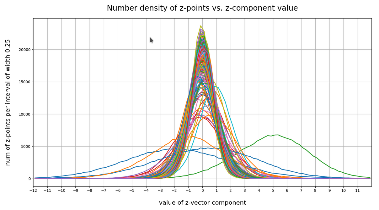
Autoencoders and latent space fragmentation – II – number distributions of latent vector components
Autoencoders and latent space fragmentation – III – correlations of latent vector components
Autoencoders and latent space fragmentation – IV – CelebA and statistical vector distributions in the surroundings of the latent space origin
Autoencoders and latent space fragmentation – V – reconstruction of human face images from simple statistical z-point-distributions?
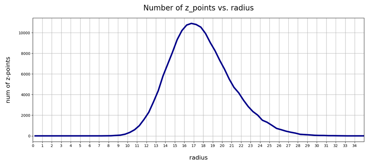
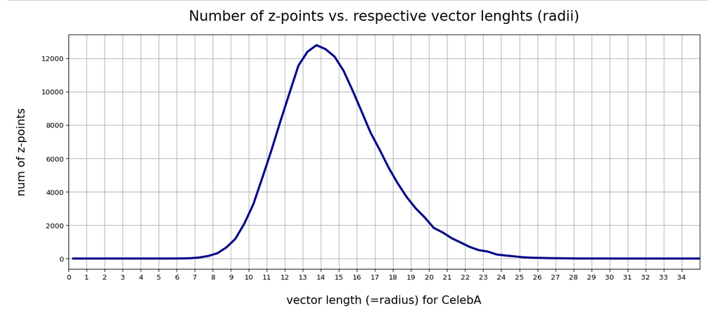
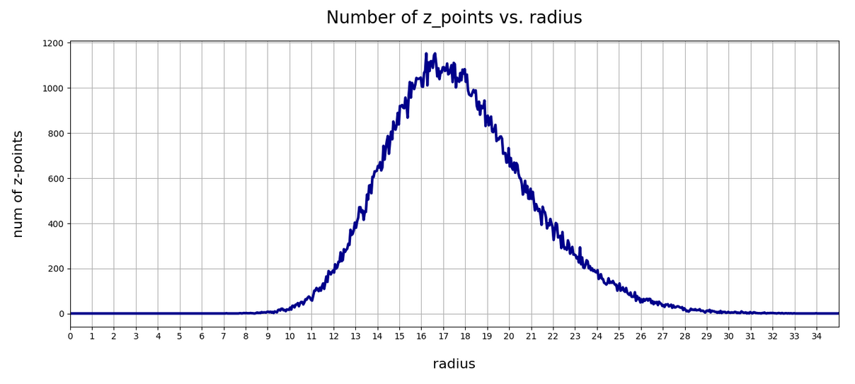
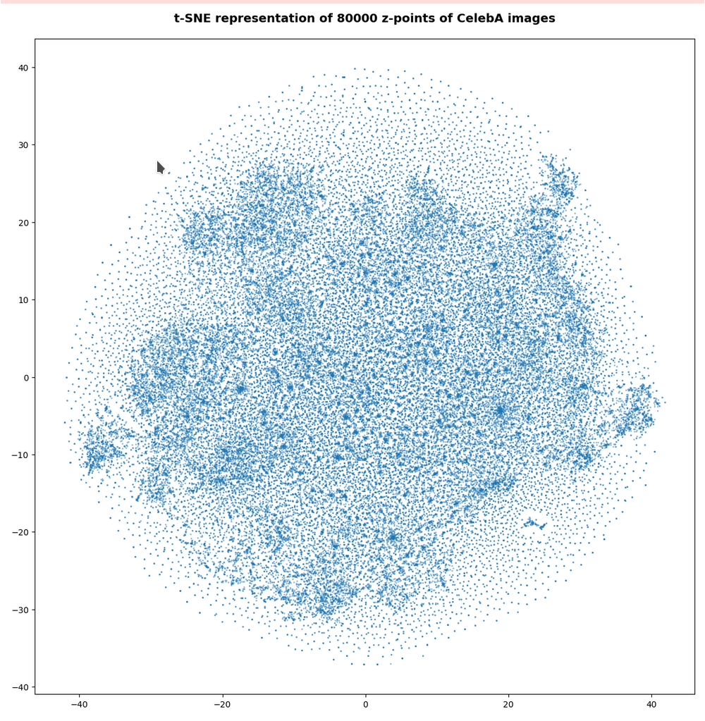
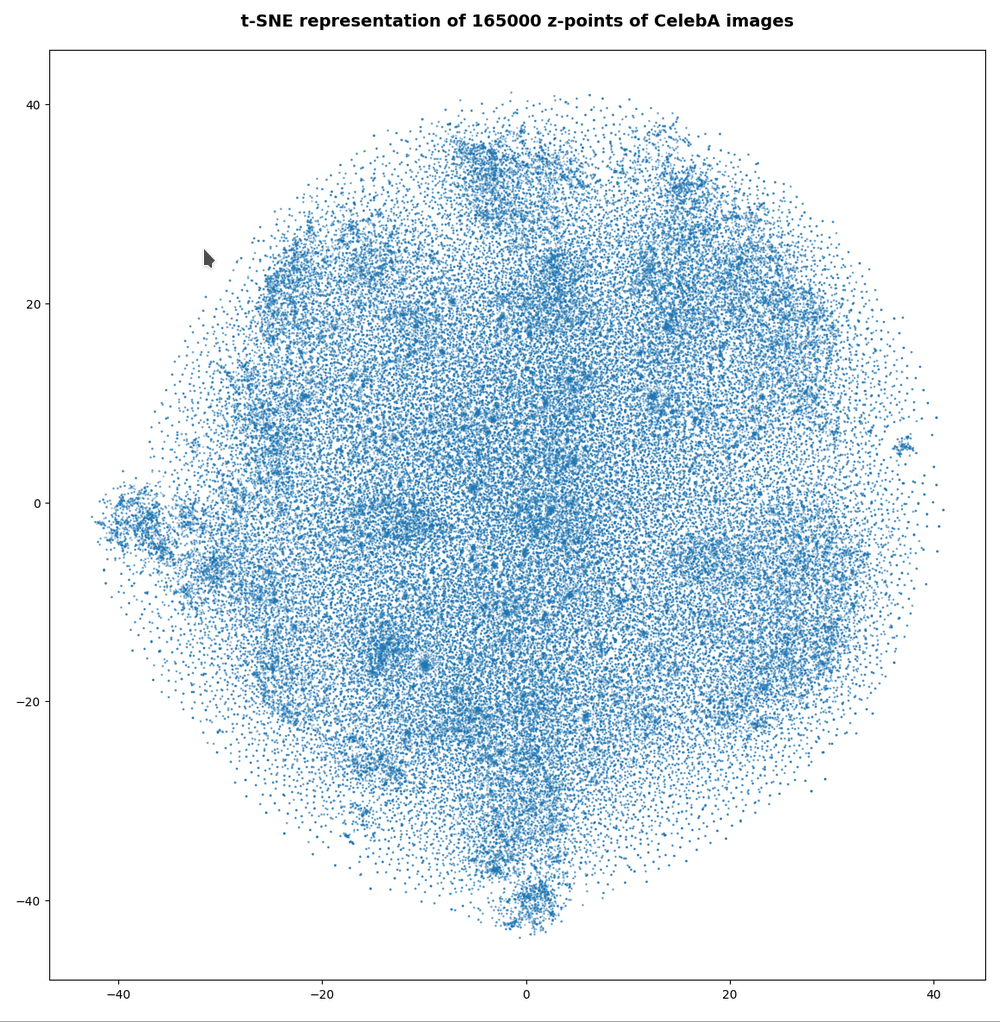
So far I have demonstrated that randomly generated vectors most often do not hit the relevant regions in the AE’s latent space – if we do not take some data specific precautions. A relevant region is a confined volume which a trained Decoder fills with z-points for its training objects after the training has been completed. z-points and corresponding latent vectors are the result of an encoding process which maps digitized input objects into the latent space. Depending on the data objects we may get multiple relevant regions or just one compact region. In the case of a convolutional AE which I had trained with the CelebA dataset of human face images I found single region with a rather compact core.
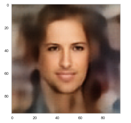
In this post I want to create statistical latent vectors whose end-points are located inside the relevant region for CelebA images. Then I will create images from such latent vectors with the help of the AE’s Decoder. My hope is to get at least some images with clearly visible human faces. The basic idea behind this experiment is that the most important features of human faces are encoded by a few dominant vector components defining the overall position and shape of the multidimensional z-point region for CelebA images. We will see that the theory is indeed valid: Here is a first example for a vector pointing to an outer area of the core region for CelebA images in the latent space:
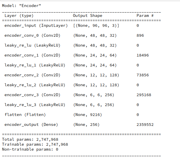
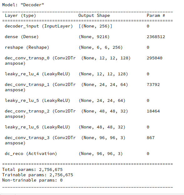
Our AE is a convolutional one. The number of latent space dimensions N was chosen to be N=256.
Note: We are NOT using a Variational Autoencoder, but a simple standard Autoencoder. The AE’s properties were discussed in previous posts.
What have we found out so far?
The Encoder of the convolutional AE, which I had trained with the CelebA dataset, mapped the human face images into a compact region of the latent space. The core of the created z-point distribution was located within or very close to a tiny hyper-volume of the latent space spanned by only a few coordinate axes. The confined multi-dimensional volume occupied by most of the z-points had an overall ellipsoidal shape with major extensions along a few main axes. We saw that some of the coordinates of the CelebA z-points and the components of the corresponding latent vectors were strongly correlated. In addition the value range of each of the latent vector components had specific individual limits – confining the angles and lengths of the vectors for CelebA. Therefore we had to conclude:
Whenever we base our method to create statistical vectors on the assumptions
- that one can treat the vector components as independent statistical variables
- that one can assign statistical values to the components from a common real value interval
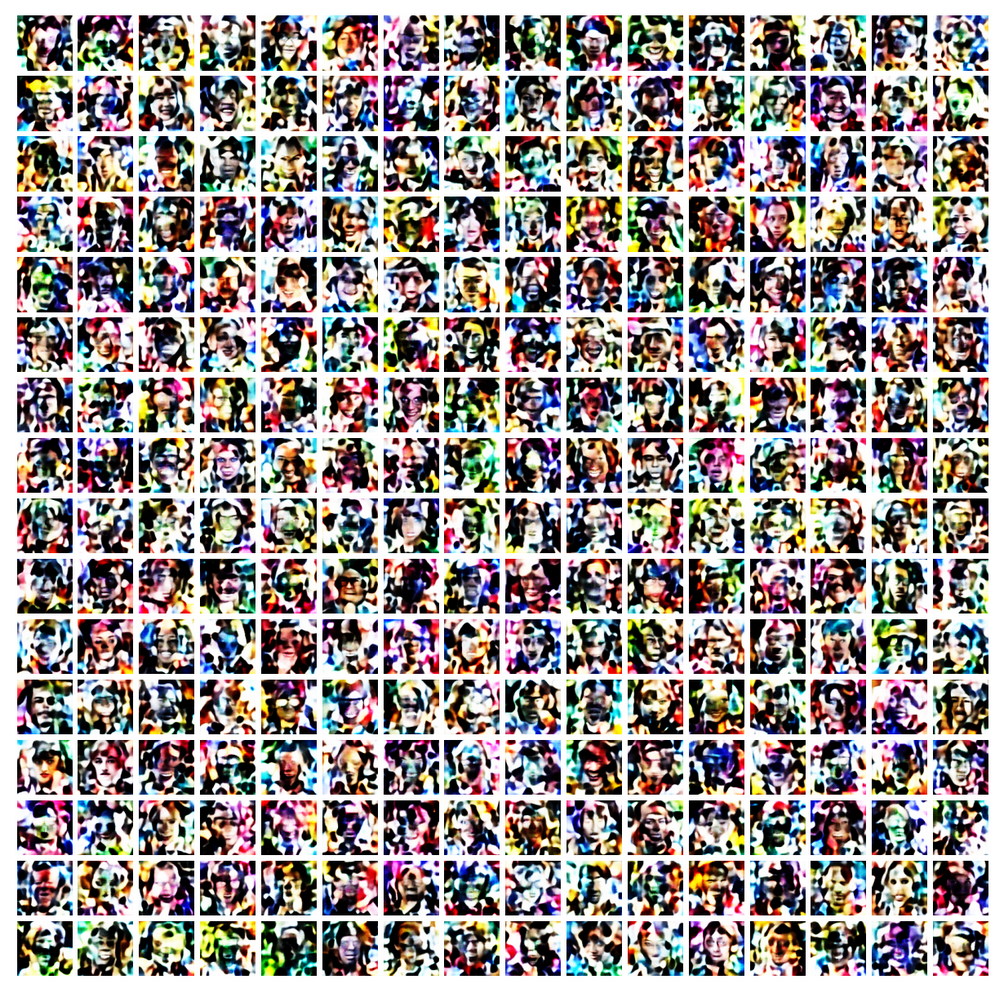
the vectors will almost certainly not point to the relevant region. In addition one has to take into account unexpected mathematical properties of statistical vector distributions in high dimensional spaces. See the previous posts for more details. Indeed we could show that such a vector generation method missed the CelebA region.
Objective of this post
In this post I want to use some of the knowledge which we have gathered about the latent vector distribution for CelebA images. We shall use a very simple approach to probe the image reconstruction abilities of the Decoder for a defined variety of z-points:
We restrict the vectors’ component values such that most of the vectors point to the region formed by the bulk of CelebA z-points. To achieve this we define straight line segments which cross the ellipsoidal region of CelebA z-points. This is possible due to the known value intervals which we have identified for each of the components in a previous post. Then we place some artificial z-points onto our line segments. At least some of these z-points will fall into the relevant CelebA region. We then let the Decoder reconstruct images for the latent vectors corresponding to these z-points.
In some cases our paths will even respect some major component correlations, but for some paths I will explicitly disregard such correlations. Nevertheless our rather simple restrictions imposed on the vector-component values will already enable us to produce images with clearly recognizable face features.
Among other things our results confirm the idea that the real pixel correlations for basic face features are represented by relatively narrow limits for the angles and lengths of respective latent vectors. The extension and shape of the bulk region of CelebA z-points is defined by only a few latent vector components. These components apparently encode a prescription for the (convolutional) Decoder to create face features by a superposition of some elementary patterns extracted during the AE’s training.
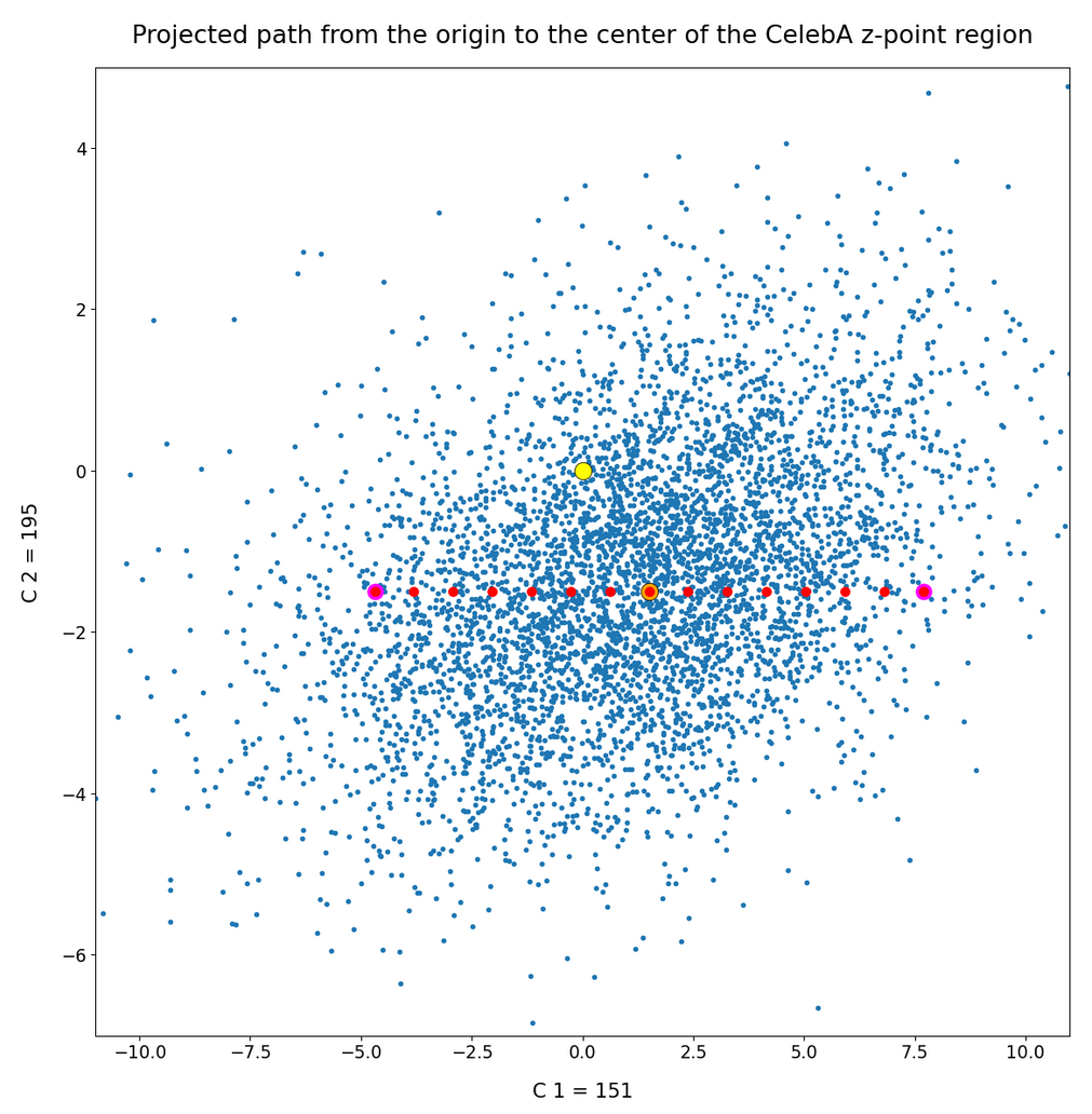
A path from the latent space origin to the center of the relevant z-point region
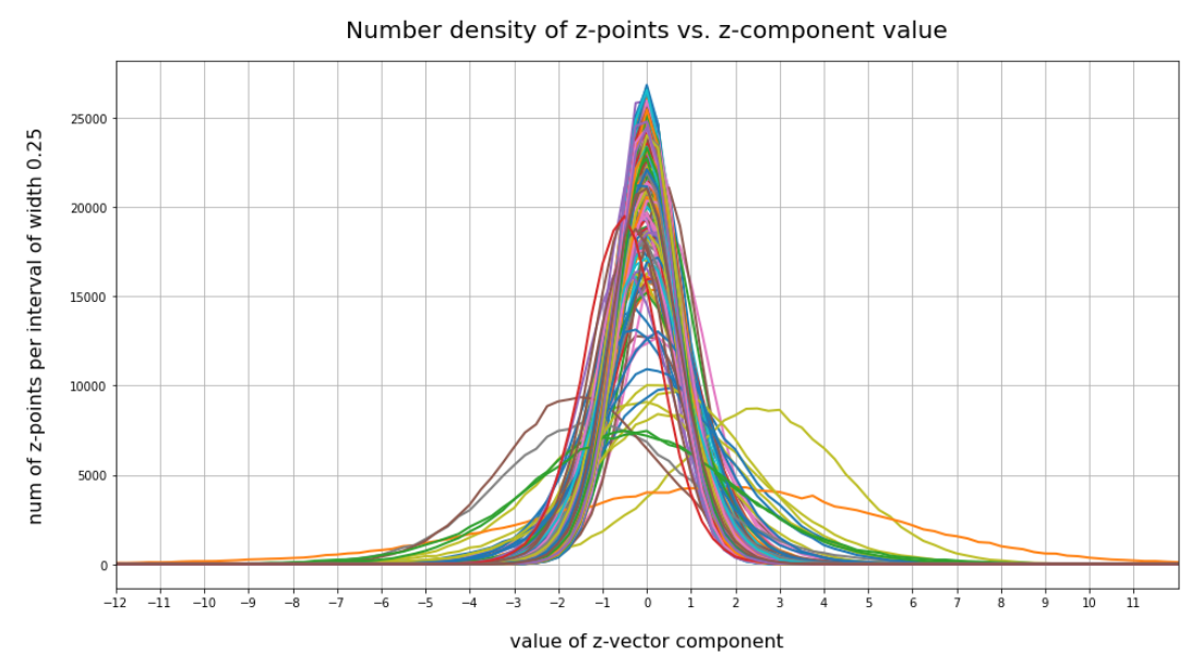
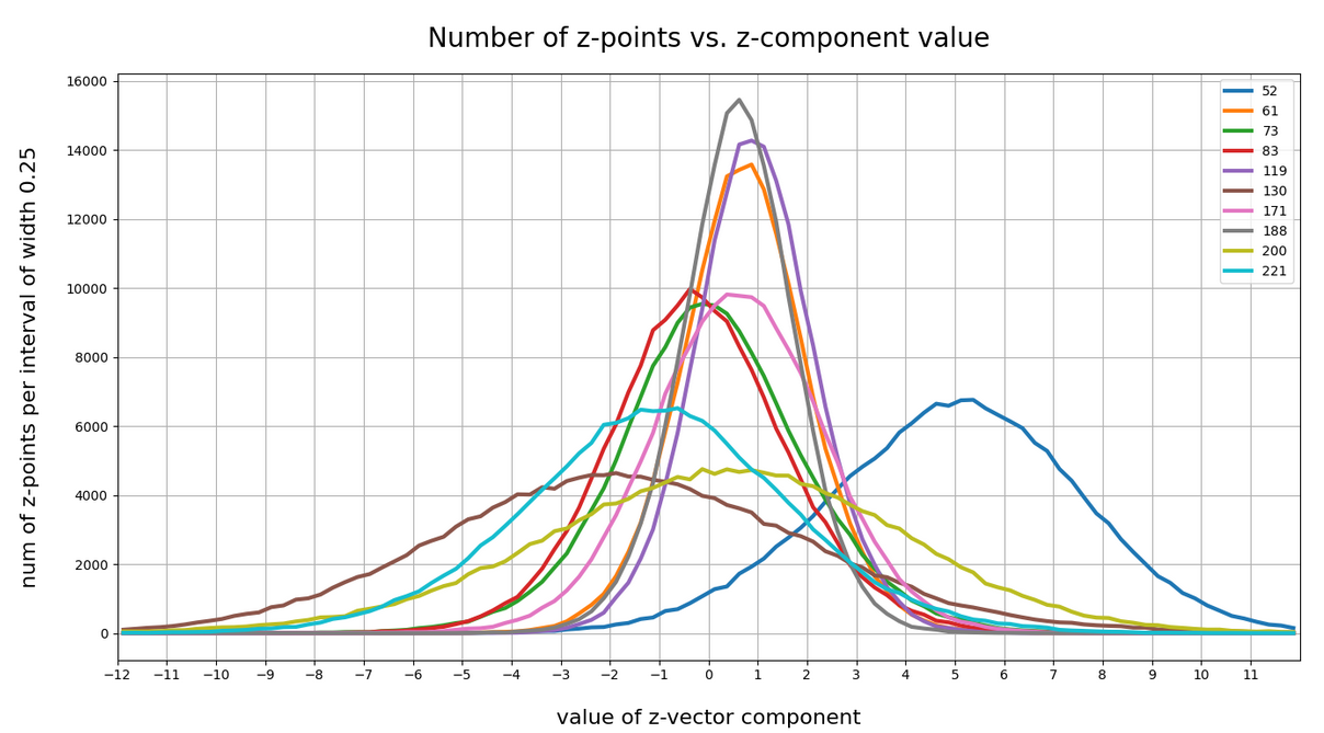
How do we restrict latent vectors to the required value ranges? In the 2nd post we have seen that the number distribution curve for the values of each of the latent vector components was very similar to a Gaussian. We have identified the mean value and average value range for each component by analyzing its specific distribution curve. The mean values gave us the coordinates of the center of the relevant latent space region. In addition we, of course, know the coordinates of the origin of the latent space. So, for a first test, let us create a multi-dimensional line segment between the origin and the center of the CelebA z-point distribution. And let the A’s Decoder create images for latent vectors pointing to some intermediate z-points along this path.
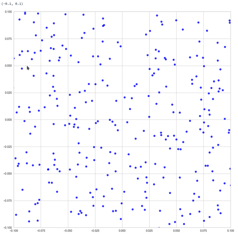
The following plots show orthogonal projections of 5000 CelebA z-points (in blue) onto some 2-dimensional planes spanned by two selected coordinate axes. The yellow dot indicates the origin. The orange dot the center of the z-point distribution. Red dots indicate coordinates of points along the straight path between the origin and the distribution center.
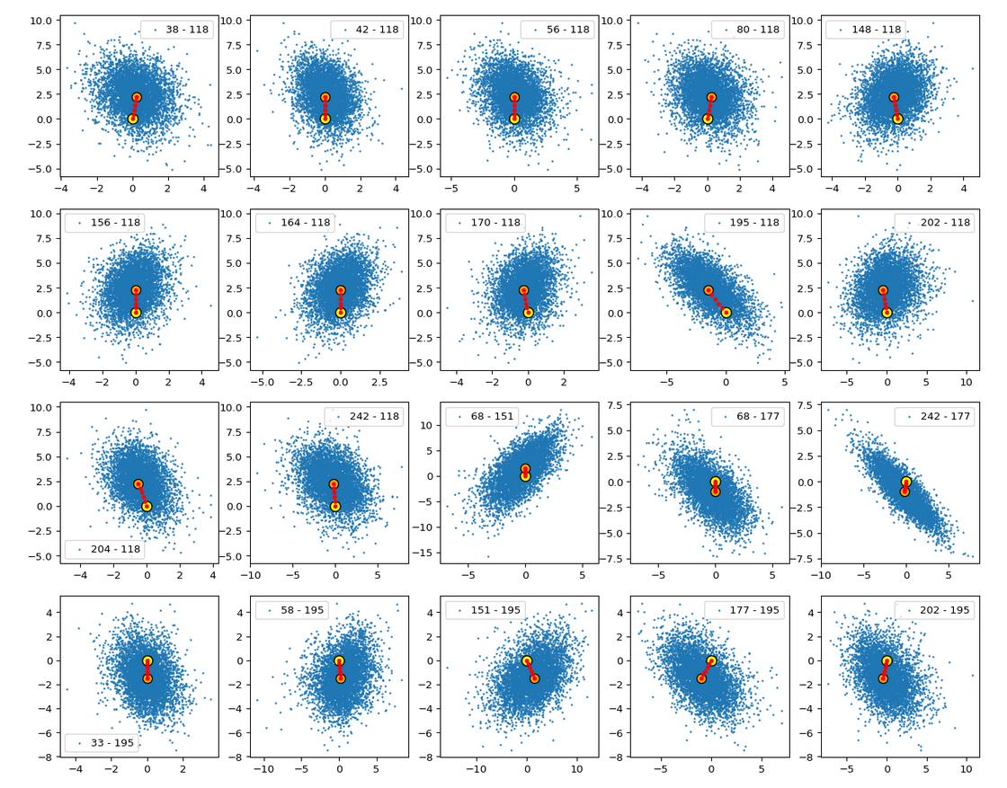
Please, take note of the different scales on the x- and y-axes. Some distributions are much more elongated than the scaled images show. That some paths appear shorter than others is due to the projection of the diagonal line through the multi-dimensional space onto planes which are differently oriented with respect to this line. A simple 3D analog should make this clear. Some small wiggles in the positions of the red dots are due to resolution problems of the plot on the browser interface. We also see a reflection of the fact that the origin is located in a border region of the bulk.
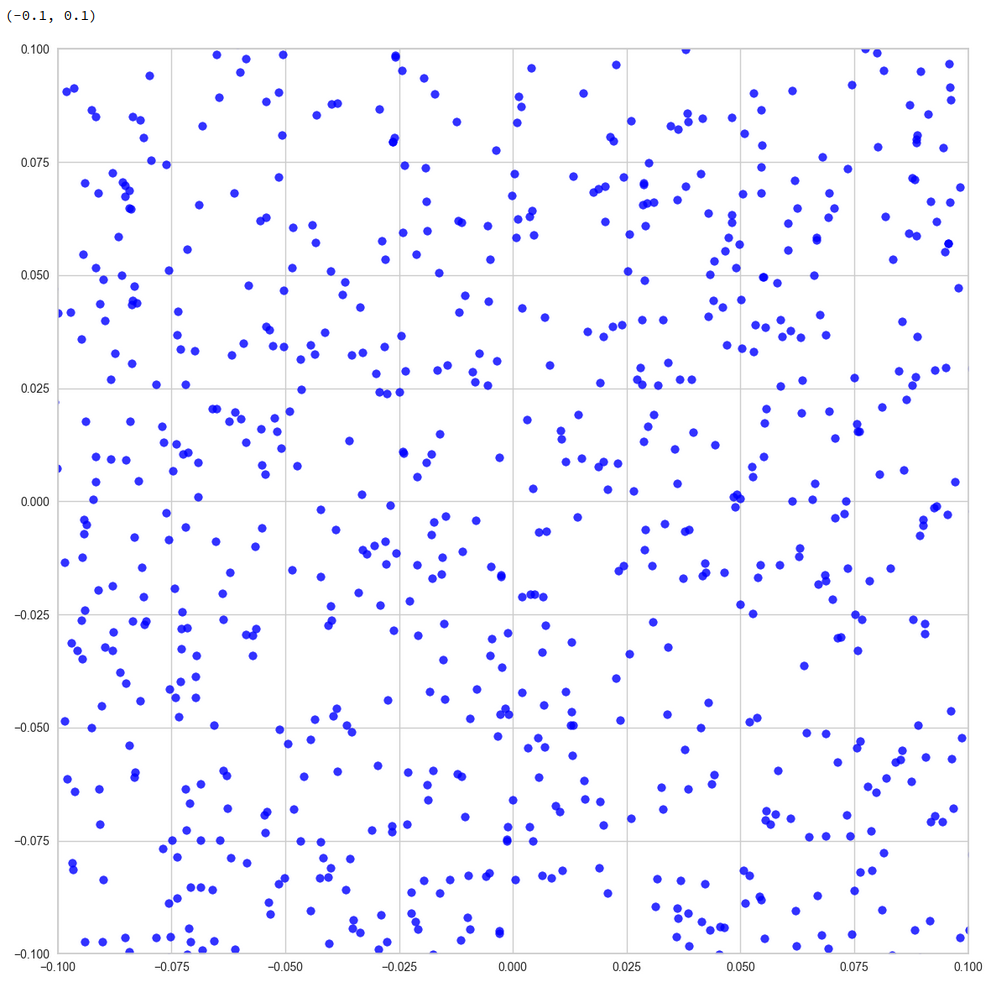
Below you see a plot which shows the path in higher resolution (projected onto a particular plane):
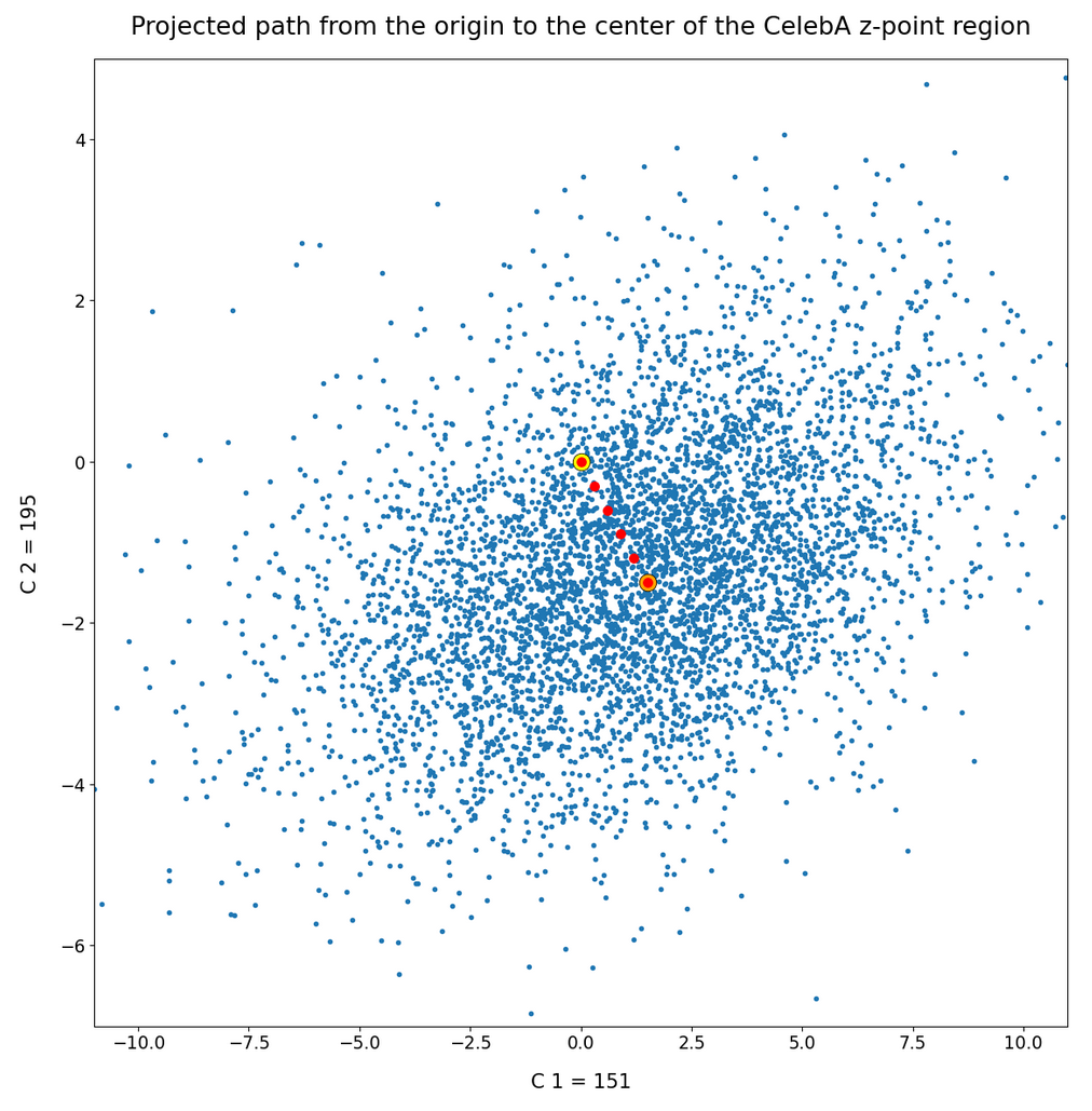
Again: Take note of the different axis scales. The blue dot distribution is much more stretched in C1-direction than it appears in the plot.
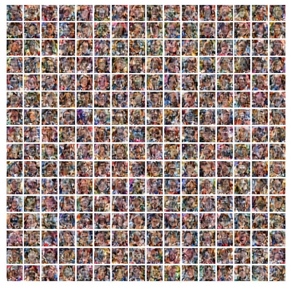
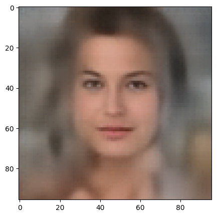
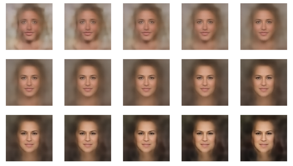
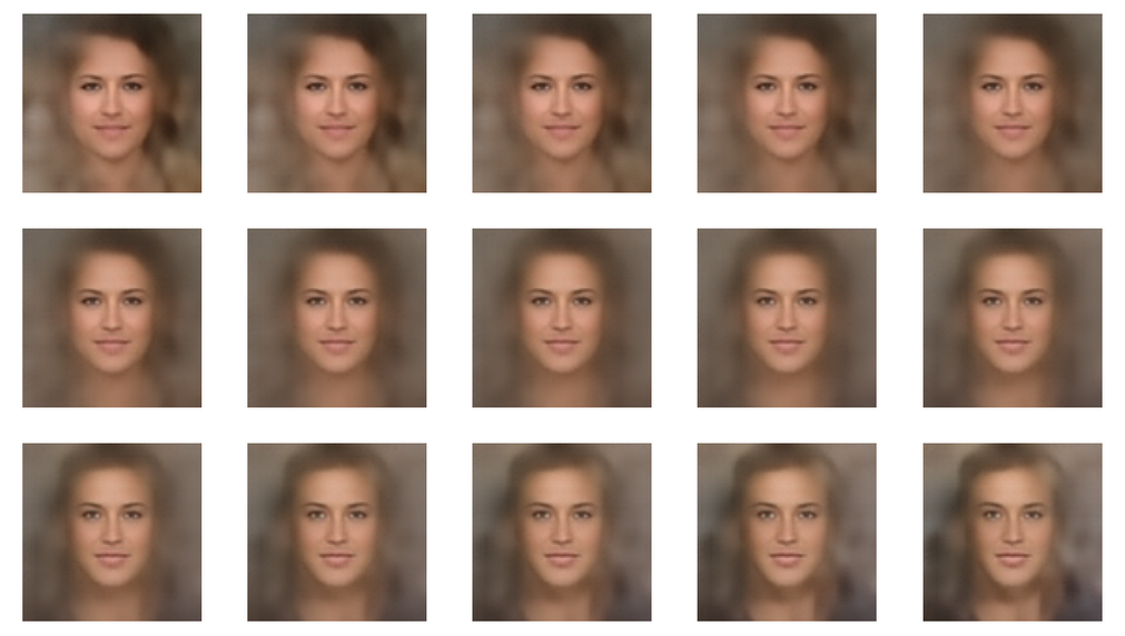
Ok, now we have a multidimensional path and six well defined latent vectors for the end and intermediate points on this path. So let us provide these vectors as input to the our AE’s Decoder. The resulting images look like:
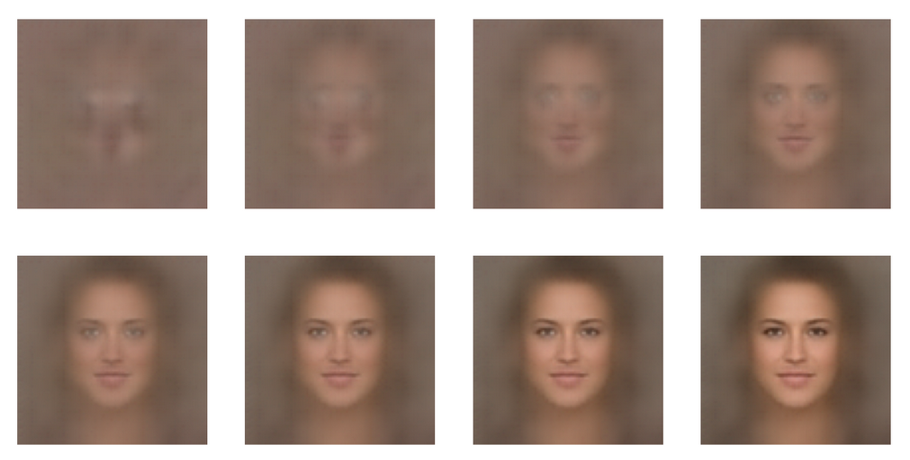
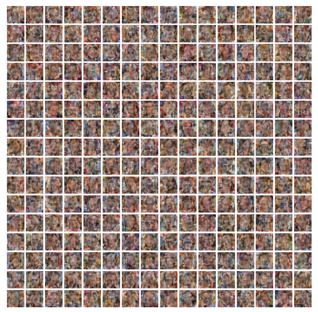
Success! Images in the surroundings of the center show a clearly visible face. And we also see: The average face at the center of the z-point distribution is female – at least according to the CelebA dataset. 🙂 However: In the vicinity of the origin of the latent space we get no images with reasonable face features.
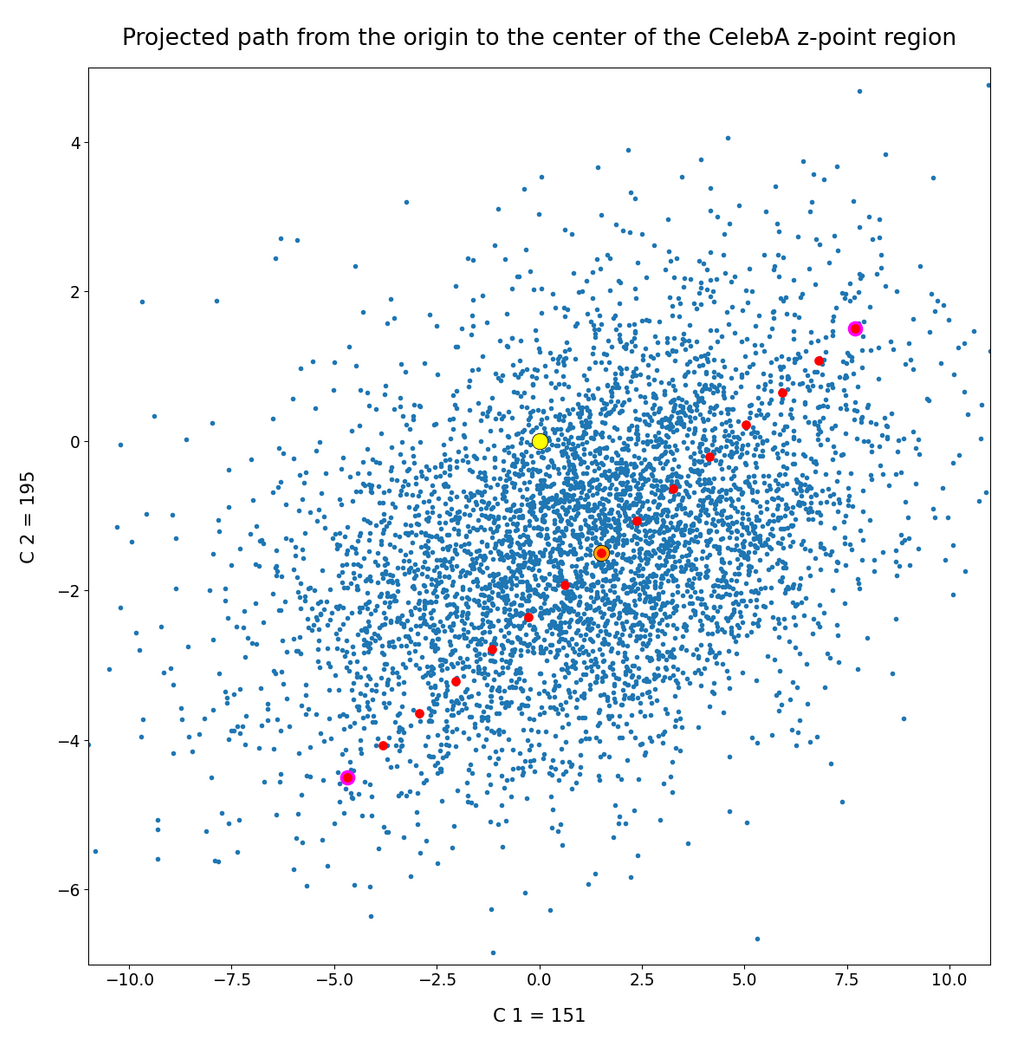
Images along a path within a selected coordinate plane for two dominant vector components
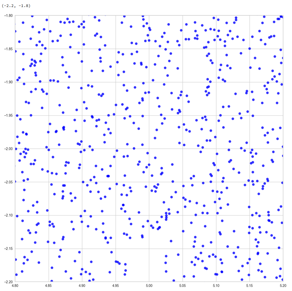
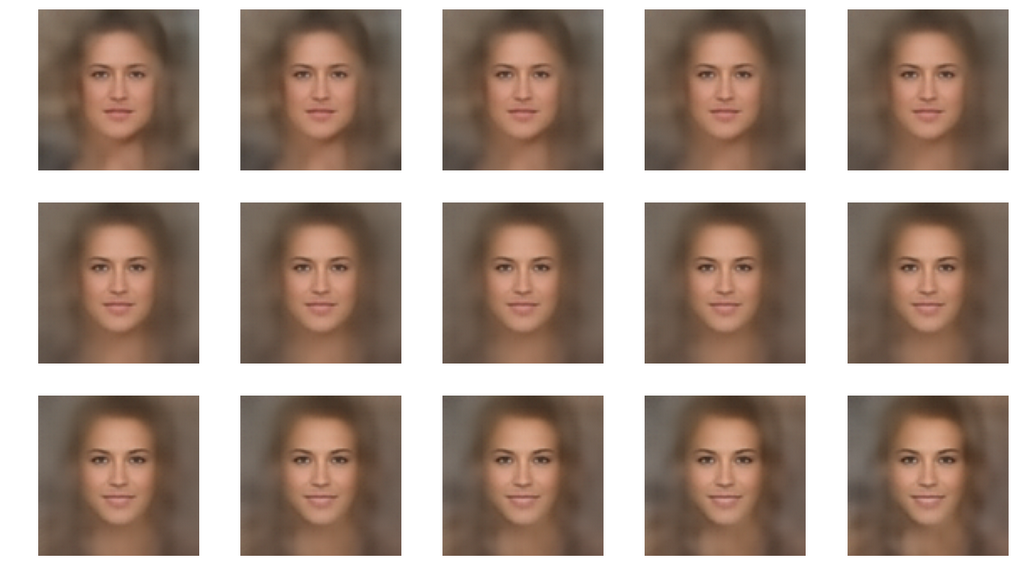
I choose a different path within the plane spanned by the coordinates axes 151 and 195 now. This is depicted in the plot below:
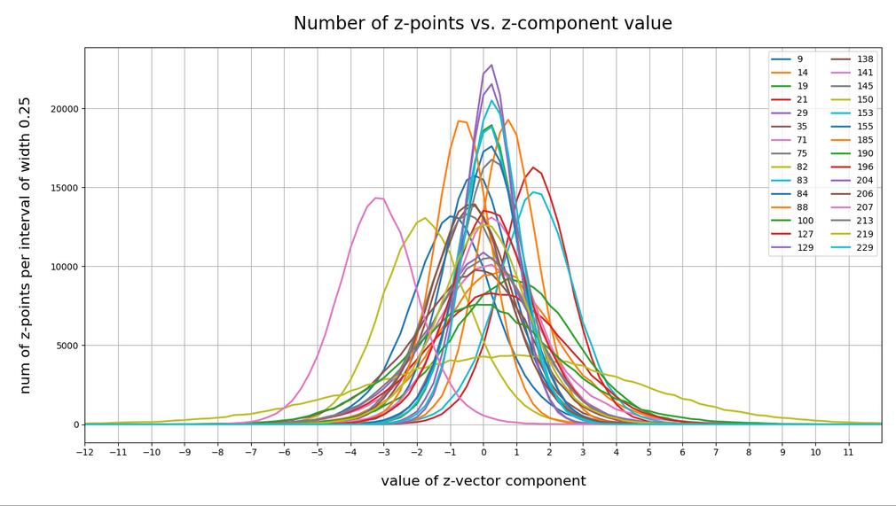
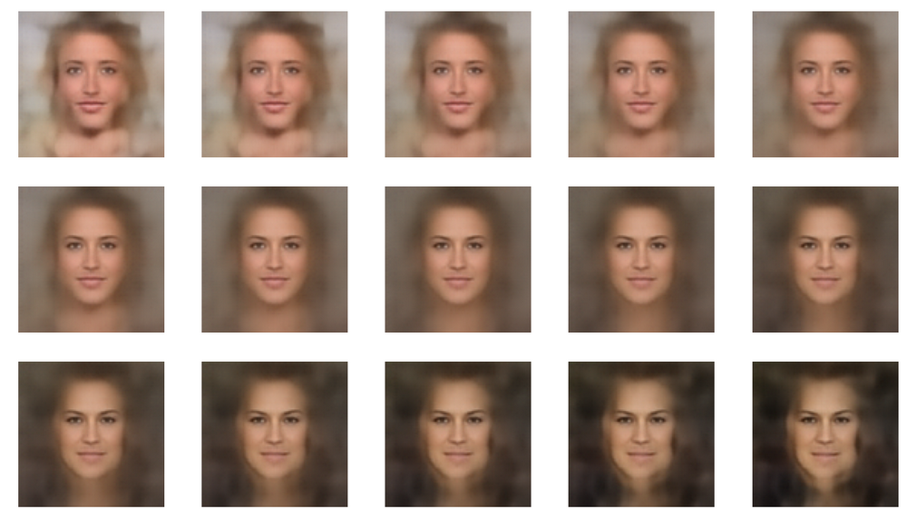
A look into the second post shows you that the components 151, 195 were members of the group of dominant components. Those were components for which the number distribution showed a mean value at some distance from the origin of the latent space and also had a half-width bigger than 1.0 (as most of the other components). The images reconstructed by the Decoder from the latent vectors are:
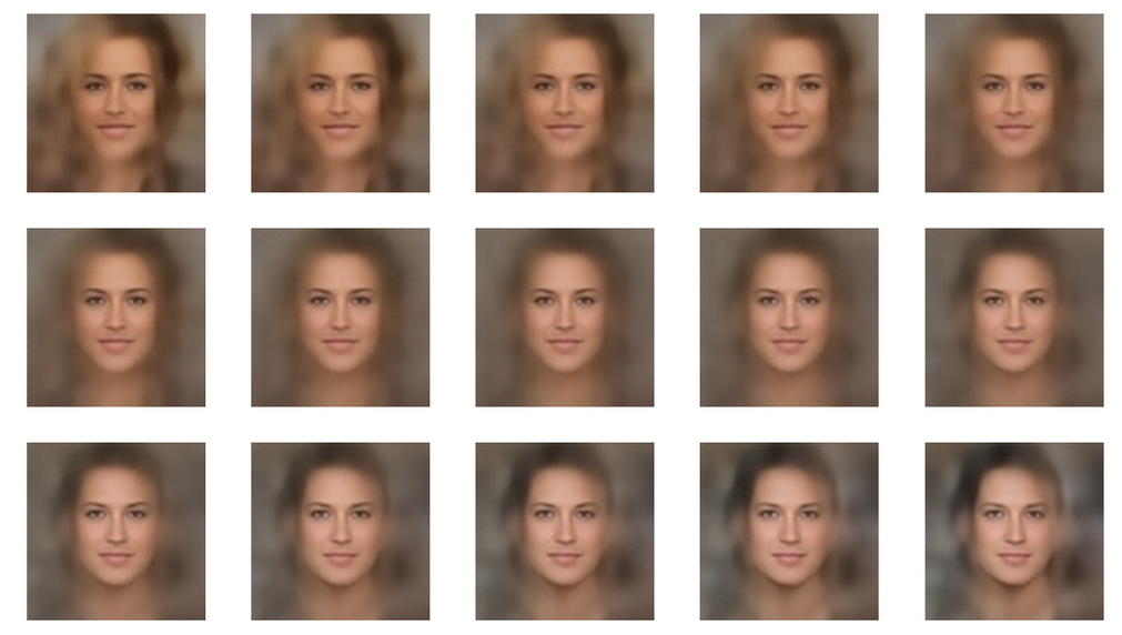
Hey, we get some variation – as expected. Now, let us rotate the path in the plane:
Not so much of a difference. But we have learned that a variation of some vector component values within the allowed range of values may give us already some major variation in the faces’ expressions.
Images for other coordinate planes
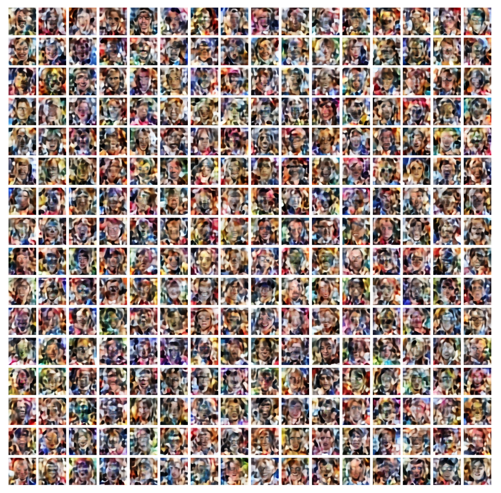
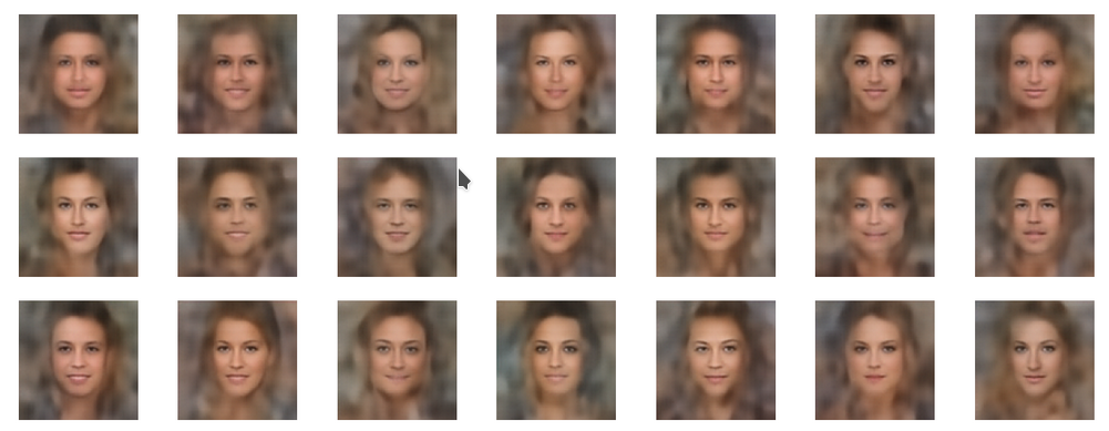
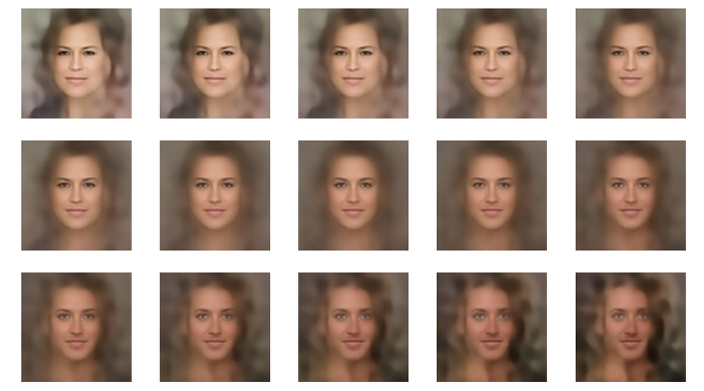
The following images show the variations for paths in other coordinate planes. All of the paths have in common that they pass the center of the CelebA bulk region. For the first 4 examples I have kept the path within the core region of CelebA z-points. The last images show images for paths with z-points at the core’s border regions or a bit outside of it.
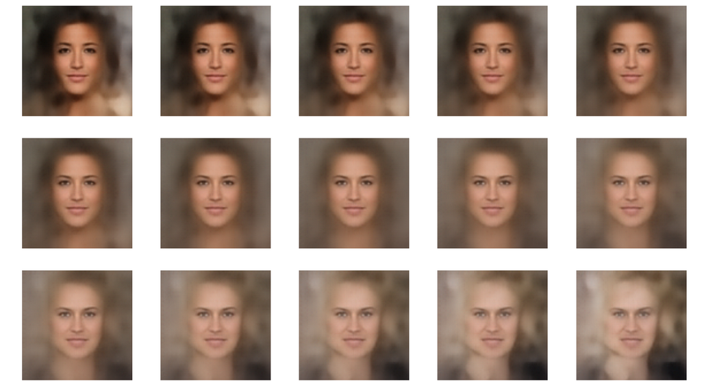
Plane axes: 5, 8

Plane axes: 17, 180
Plane axes: 44, 111
Plane axes: 55, 56
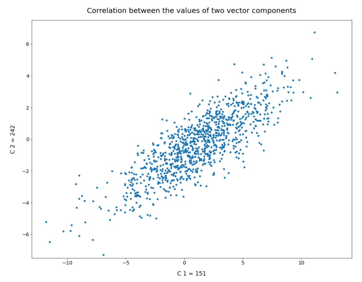
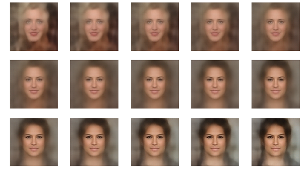
Plane axes: 15, 242
Plane axes: 58 202
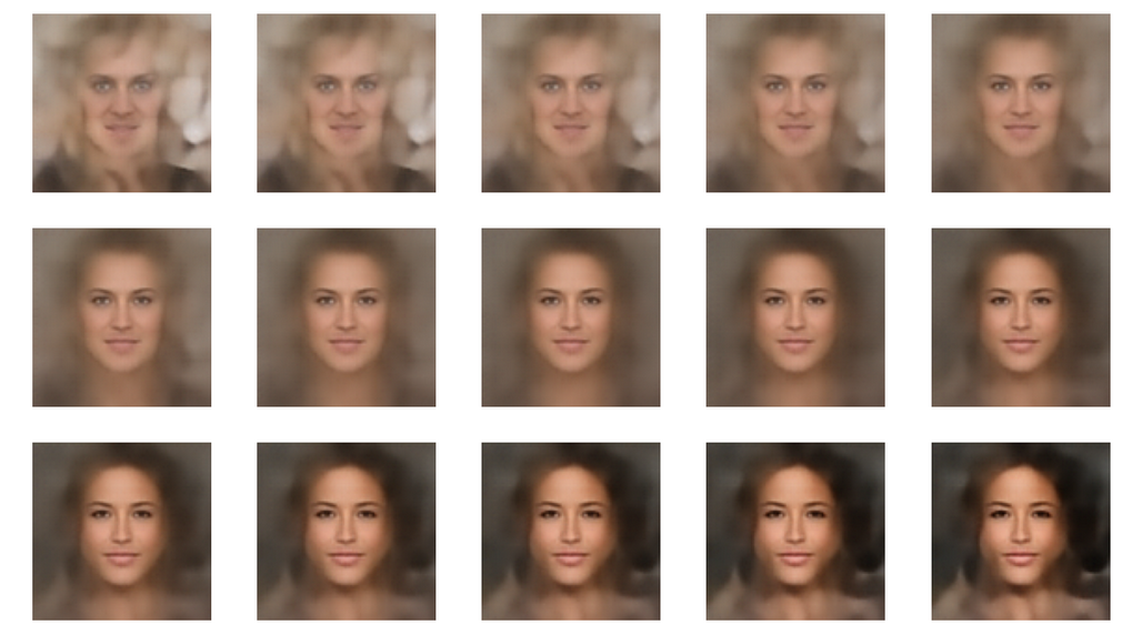
Plane axes: 68, 178
Plane axes: 177, 202
Plane axes: 180, 242
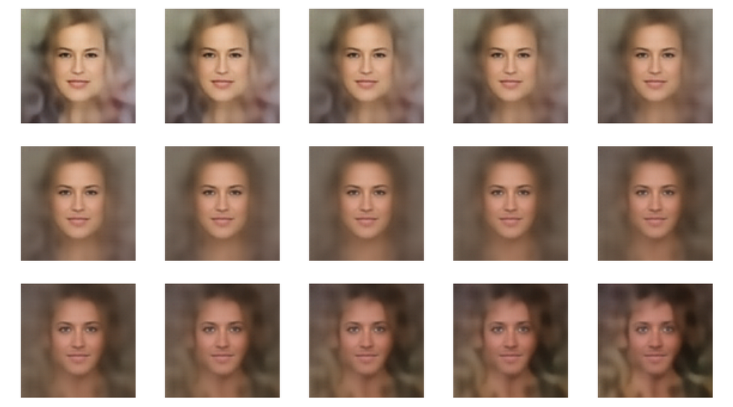
The images for z-points farther away from the bulk’s center give you more interesting variations. But obviously in the outer areas of the CelebA region correlations between the latent vector components get more important when we want to avoid irregular and unrealistic disturbances. All in all we also get the impression that a much more subtle correlation of component values is a key for the reproduction of realistic transitions for the hairdos presented in the CelebA images and the transition to some realistic background patterns. The components of our latent vectors are still too uncorrelated for such details and an appropriate superposition of micro-patterns in the images created by the Decoder.
Conclusion
This blog shows that we do not need a Variational Autoencoder to produce images with recognizable human faces from statistical latent vectors. We can get image reproductions with varying face features also from the Decoder of a standard convolutional Autoencoder. A basic requirement seems to be that we keep the vector components within reasonable value intervals. The valid component specific value ranges are defined by the shape of the compact hyper-volume, which an AE’s Encoder fills with z-points for its training objects. So we need to construct statistical latent vectors which point to this specific sub-region of the latent space. Vectors with arbitrary components will almost certainly miss this region and give no interpretable image content.
In this post we have looked at vectors defining z-points along specific line segments in the latent space. Some of the paths were explicitly kept within the inner core regions of the z-point-distribution for CelebA images. From these z-points the most important face features were clearly reconstructed. But we also saw that some micro-correlations of the latent vector components seem to control the appearance of the background and the transition from the face to hair and from the hair to the background-environment.
I have not yet looked at line segments which do not cross the center of the bulk of the z-point distribution for CelebA images in the latent space. But in the next post
I first want to look at z-points for which we relatively freely vary the component values within ranges given by the respective number distributions.