Latent spaces – pitfalls of distributing points in multi dimensions – I – constant probability density per dimension

This post requires Javascript to display formulas!

Sometimes when we solve some problems with Deep Neural Networks we have no direct clue about how such a network evolves during training and how exactly it encodes knowledge learned from patterns in the input data. The encoding may not only affect weights of neurons in neural filters or maps, but also the functional mapping of input data onto vectors of some intermediate or target vector space. To get a better understanding it may sometimes seem that experiments with statistical points or vectors in such vector spaces could be helpful. One could e.g. suggest to study the reaction of a trained Artificial Neural Network to input vectors distributed over a multidimensional feature space.

Another important case is the test of an Autoencoder’s Decoder network on data points which we distribute statistically over extended regions of the Autoencoder’s latent space.

An Autoencoder [AEs] is an example of a Encoder-Decoder pair of networks. The Encoder encodes original complex input data into vectors of the so called latent space – a multi-dimensional vector space. The Decoder instead uses vectors of the latent space to reconstruct or generate output data in the feature space of the original input objects. The dimensionality of the latent space may be much smaller than that of the original feature space, but still much bigger than the 2 or 3 dimensions we have intuitive experience with.

Latent spaces play a major role in Machine Learning [ML] whenever a deep neural algorithm encodes information. Embedding input data (like words or images) in a vector space by some special neural layers (e.g. for text or image classification) is nothing else than filling a kind of latent space with encoded data in an optimized way to help the neural network to solve a special task like e.g. text or image classification. But we can also use statistical data in the latent space of an AE together with its trained Decoder to create or better generate new objects. This leads us into the field of using neural networks for generative, creative tasks.

Unfortunately, we know from experience that not all data regions in a latent space support the production of objects which we would consider as being similar to our training objects or categories of such objects. A priori we actually know very little about the shape of the data distribution an encoding network will create during training. Therefore we may be tempted to scan the latent space in some way – and to distribute data points in it in some statistical way. And test a Decoder’s reaction to such points …in the hope to find an interesting region by chance.

In this small series of posts I want to point out that such statistical experiments may be futile. On the one hand side trying to fill a multidimensional space with “statistical” data may lead to unexpected and counter-intuitive results. On the other hand side you may easily miss interesting regions of such a vector space. Especially confined regions. The whole point is just another interesting variant of the curse of high dimensions.

The theoretical and numerical results which we will derive during the next posts underline the necessity to analyze the concrete data distributions a neural network creates in a latent space very carefully. Both regarding position and extension of the filled region – and maybe also with respect to sub-structures. The results will help us to understand better why an Autoencoder most often fails to produce reasonable objects from data points statistically distributed over larger regions of its latent space.

This post series requires an understanding of some basic math. In the first post I will derive some formulas describing data distributions resulting from a constant probability density for each vector component, i.e. a constant probability density per dimension. We will learn that with a growing number of dimensions the data points concentrate more and more in regions which are parts of a multi-dimensional sphere shell. Which is at least in my opinion a bit counter-intuitive and therefore an interesting finding in itself.

Many dimensions …

An AE compresses data very effectively. So the dimension of a latent space will most often be significantly smaller than the number of dimensions M characterizing the feature space of the original training objects. The space spanned by logically independent variables which describe digitized objects may have a number of dimensions in the range of millions and tenths of millions. In the case of latent spaces we instead have to deal with a number of dimensions N in the range of multiples of 10 up to tens of thousands. (For relatively simple objects showing many correlations in their feature space …)

10 ≤ N ≤ 105    << M

Still, such numbers N are far beyond standard experience.

Representation of a N-dimensional space by the ℜN

We can in general represent a multidimensional feature or latent space in Machine Learning by the ℜN. Each point in this space can be defined by a vector whose components correspond to the points’ coordinate values along the N orthogonal axes. A vector is thus represented by a N-tuple of real (coordinate) values:

(x1, x2, …, xk, … xN) .

Formally, the set of all tuples together with some addition and multiplication operations form a vector space over ℜ. Whether vector operations performed with vectors to different data points in a latent space or a feature space really have a solid interpretable meaning in your ML- or AE-context is not our business in this post. Our objective is to cover such a space with statistically defined points (or vectors).

The curse of high dimensionality

It seems to be easy to fill a N-dimensional cube with data points that form a grid. More precisely, a grid with a constant distance between the points in all orthogonal directions parallel to the axes. However, a simple calculation shows that such an approach is doomed in computational practice:

Let us assume that we deal with a space of N = 256 dimensions. Let us also assume that we have reasons to believe that we should focus on the region of a cube around the origin that has a side length of 10 in each dimension k. Then the coordinate values xk for data points within the cube fulfill

\[ -b \lt x_{k} \lt +b \mbox{,} \quad \forall k \: \in [1,256] \quad \mbox{and} \quad b=5
\]

Let us further assume that we want to have a grid resolution of 10 points per dimension. Then we would need to create

\[ 10^{256} \: \mbox{points}
\]

to fill our 256-dimensional cube with a homogeneous (!) point distribution. This is already a very clear indication that we can not systematically study a multidimensional cube in this way. Multidimensional spaces are huge by their nature.

We have to get and use more information about interesting regions or we must make assumptions on the distribution of points in each coordinate direction.

Constant probability density per coordinate value and dimension

A most simple case for making an assumption is a constant probability distribution of each coordinate value xk within a defined interval along the related coordinate axis. Let us again pick a cube around the origin of a space with N=256:

\[-b \lt x_{k} \lt +b, \quad \forall k \: \in [1,256] \quad \mbox{and} \quad b=5 \]

Let us assume that we only want a resolution of 100 equidistant values per side length of the cube. From a statistical point of view we deal with our dimensions like they were part of a classical experiment in which we pick balls with imprinted values from a (mixing) black box. In our assumed case we have a box with 100 numbers and fetch a ball 256 times to create a 256-tuple for each vector – of course with laying back the picked ball each time. We will come back to this interpretation in a second post. For now let us define a constant probability density and see where we get from there mathematically.

The normalized density distribution in the interval [-b, b] simply is

\[ \rho(x_k) \: = \: \frac{1}{2b} \:, \quad \mbox {for} \: -b \le x_k < b . \]

One may “naively” think the following:
We statistically fetch 256 xk-values, each from our uniform distribution, and fill our vector N-tuples with these values. Repeating this vector generation process for e.g. 200000 times should give us some widespread point distribution covering our cube very well. Let me warn you:

This is a common mistake – although such a procedure seems to work rather well in 2 or 3 dimensions!

It admit: The whole thing is somewhat counter-intuitive. If you create a homogeneous distribution for each of the coordinate values xk then the points should well cover the whole space? The answer unfortunately is: No.

To get a better understanding we need some more math. And we first reduce the problem to statements about a one-dimensional quantity, namely the vector length. But let us first look at results in 3 dimensions.

Point distribution in a 3-dimensional cube for a constant probability density of each coordinate value

Let us create some 200 points in a cube

\[ 0 \lt x_{k} \lt +b, \quad \forall k \: \in [1,3] \quad \mbox{and} \quad b=10 \]

The following plots show the distributions projections on the planes between the coordinate axes:
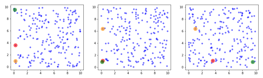
This looks quite OK. All areas seem to be covered. I have marked some points to illustrate their positions. We see that filling a corner in 2D does not necessarily mean that the points are close to the origin of the 3D coordinate system. Now, let us look at a 3D-plot:
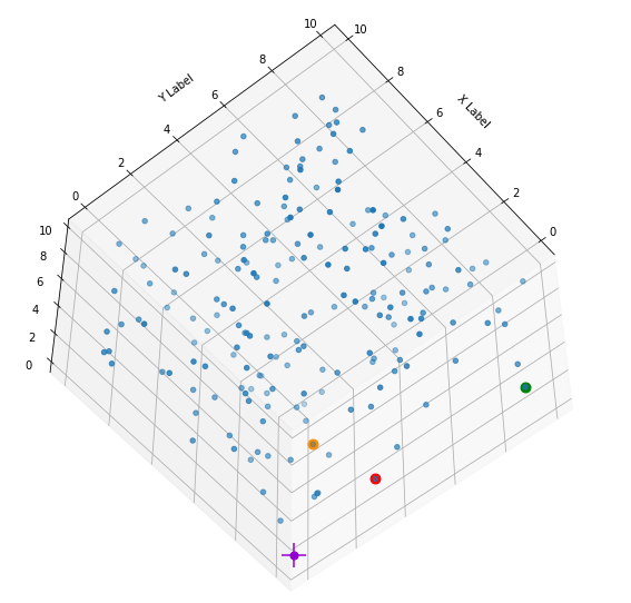
I have marked the origin in violet. Notably, extended elongated stripes at the edges with two coordinate close to extreme values seem strangely depleted. This is no accident. Below you find a similar plot with 400 points and b=5:
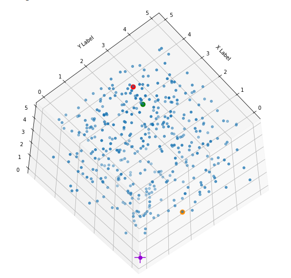
What is the reason? Well, it is simply statistics: To fill the special regions named above you have to fix one or two coordinates at the same time. Let us look at a stripe stretching from one corner and parallel to an axis and perpendicular to the plane {x_1, x_2}:

\[ x_1 \in [0,1] \: \mbox{and} \: x_2 \in [9,10], \quad \mbox{for} \:\: b=10 \]

As we deal with a uniform distribution per coordinate value the chances are 1/10 * 1/10 = 1/100 that a randomly constructed point will fulfill these conditions.

Also: For a region with all coordinates around [0,1] the chance is just 0.13 = 0.001.

When see already that the probability to get a point with a limited radius vector becomes rather small. Now, what happens in a real multi-dimensional space, e.g. with N=256?

The mean radius of data points created with a constant probability density for each coordinate value

Let us call the length of a vector directed from the origin to some defined point in our cube the “radius” R of the vector. This radius then is defined as:

\[ R \: = \: \sqrt{\,\sum_{k=1}^{N} (x_k)^2 \,} \]

What is the length of a vector with all xk = 1 for all k? For N=256 dimensions the answer is:

\[ R = \sqrt{256} \: = 16 \: \]

So, we should not be surprised when we have to deal with large average numbers for vector lengths in the course of our analysis below. We again assume a constant probability density ρ along the each coordinate axis in the interval [-b, b]

\[ \rho(x_k) \: = \: \frac{1}{2b} \:, \quad \mbox {for} \: -b \le x_k < b . \]

Now, what will the mean radius of a “random” point distribution in the cube be when we base the distribution on this probability density? How do we get the expectation value <R> for the length of our vectors?

If we wanted to approach the problem directly we would have to solve an integral over the vector length and a (normalized) probability density. This would lead us to integrals of the type

\[ \lt R \gt \: = \: \int_{-b}^{b}\int_{-b}^{b}…\int_{-b}^{b}\, \rho_N(x_1, x_2, …x_{N}) * \sqrt{ \sum_{k=1}^{256} (x_k)² }\:\: dx_1\,dx_2…\,dx_{N} \]
\[ \rho_N(x_1, x_2, …x_{N}) = \rho(x_1) * \rho(x_2) * … * \rho(x_N) \]

As our normalized probability density per dimension is a constant, the whole thing looks simple. However, the integrals over the square root are, unfortunately, not really trivial to handle. Try it yourself …

Therefore, I choose a different way: Instead of looking for the expectation value of the vector length <R> I look for the square root of the expectation value of the vector length squared R2 – and assume:

\[ \lt R \gt \: \approx \: \sqrt{\lt R^{\,2} \gt\,} \quad . \]

We take care of this assumption later by giving a reference and an approximation formula.

We also use the fact that the expectation value is a linear function for a sum of independent quantities. This leads us to

\[ \lt R^{\,2} \gt \: = \: \sum_{k=0}^{N} \lt (x_k)^2 \gt \]

The resulting integral is much easier to solve. It splits up into simple 1-dimensional integrals. Note: Each of your squared coordinate values (xk)2 is associated with a simple, un-squared (!) probability density of 1/(2b) for an interval [-b, b] or 1/(b-a) for [a, b].

The result for a general common interval [a,b] for all coordinate values a \le; xk ≤ b is :

\[ \lt R^{\,2} \gt \: = \: \frac{b³ \, – \, a³}{3\, ( b \, – \, a )} * N \quad .
\]

So, for our special case a = -b we get:

\[ \lt R \gt \: \approx \: \sqrt{\lt R^{\,2} \gt} \: = \: b * \sqrt{ 1/3 * N \,}
\]

This will give us for b = 5:

\[ R_{mean} = \lt R \gt \: \approx \: \sqrt{\lt R^{\,2} \gt} \: \approx \: 46.188 , \quad for N=256, b=5 \]

Note that

\[ \sqrt{1 / 3} \: \approx \: 0.57735 \: \gt \: 0.5 \]

Ok, the mean length value is a bit bigger than half of the length which a diagonal vector from the origin to the outmost edge of our cube (b, b,,…,b) would have. This does not say so much about the point and the radius distributions themselves. We have to look at higher momenta. Let us first look at the variance and standard variation for R2.

Variance and standard deviation of R2

What we actually would like to see is the variance and standard deviation for R. But again it is easier to first solve the problem for the squared quantity. The variance of R2 is defined as:

\[ \mbox{Variance of } \: R^{\,2} \:\: : \:\: \left< { \, \left( \, R^{\,2} \, – \, \lt R^{\,2} \gt \right)^{2} \, } \right>
\]
\[ \mbox{Standard deviation of } R^{\,2} \:\: : \:\: \sqrt{ \left< {\, \left( \, R^{\,2} \, – \, \lt R^{\,2} \gt \, \right)^{2} \, } \right> \,}
\]

We can solve this step by step. First we use:

\[ \left< { \,\, {\left( \, R^{\,2} \, – \, \lt R^{\,2} \gt \right)}^{2} \,\, } \right> \: = \: \left< { \, \left( R^{\,2} \right)^{2} \, } \right> – \left( \lt { R^{\,2} } \gt \right)^{2}
\]

We evaluate (for our cube):

\[ \left< { \,\, {\left( R^{\,2} \right)^{2}} \,\, } \right> – \left( \lt { R^{\,2} } \gt \right)^{2} \: = \: \left< { \,\, \left( R^{\,2} \right)^{2} \,\, } \right> \: – \: {1 \over 9} N^{\,2} \, b^{\,4}
\]

and

\[ \left< { \,\, \left( R^{\,2} \right)^{2} \,\,} \right> \: = \: \left< { \,\, \left( \sum_{k=1}^N (x_k)^{\,2} \,\right)} * {\left( \sum_{m=1}^N (x_m)^{\,2} \,\right) \,\,} \right>
\]

For the different contributions to the expectation values we get

\[ \left< { \,\, \left( R^{\,2} \right)^{2} \,\,} \right> \: = \: N * \left< { \,\, (x_k)^{\,4} \,\, } \right> + N(N-1) * \left< { \,\, (x_i)^{\,2}\,(x_k)^{\,2} \,\, } \right>
\]

Integrating over our constant probability densities for the independent coordinates gives

\[ \left< { \,\, \left( R^{\,2} \right)^{2} \,\,} \right> \: = \: N {1 \over 5} b^{\,4} \, + \, N^{\,2} {1\over 9} b^{\,4} \, – \, N {1 \over 9} b^{\,4}
\]

Thus

\[ \left< {\left( R^{\,2} \right)^{\,2}} \right> – \left( \lt R^{\,2} \gt \right)^{\,2} \: = \: N \, b^{\,4} * \left( {1 \over 5} – {1\over 9} \right) \: = \: {4 \over 45} N * b^{\,4} \: .
\]

Eventually, we get for the ratio of the standard variation of R2 to <R2> :

\[ {1 \over {\left< { \, \left( \, R^{\,2} \right)^{2} \, } \right>} } * \sqrt{ \left< \, \left( \, R^{\,2} \, – \lt R^{\,2} \gt \, \right)^{2} \, \right> \,} \: = \: { 3 \over {N * b^{\,2} }} * \sqrt{{4 \over 45} N \, b^{\,4} \,} \: = \: 2 * \sqrt{ 1 / ( 5 N) \, }
\]

The ratio of the standard variation of R to <R>

We are basically interested in the ratio

\[ {1 \over {\left< R \right>} } * \sqrt{ \left< \, \left( { \, R \, – \lt R \gt \, } \right)^{2} \, \right> \,}
\]

Before you start to fight the complex integrals over square roots think of the following:

\[ {1 \over 2} * { { \left( R_0 + \Delta \right)^{\,2} \, – \, \left( R_0 – \Delta \right)^{\,2} } \over {{R_0}^{\,2}} } \: = \: 2 { \Delta \over R_0}
\]

From an adaption of this argument we conclude

\[ {1 \over {\left< R \right>} } * \sqrt{ \left< \, \left( \, R \, – \lt R \gt \, \right)^{2} \, \right> \,} \: \approx \: \sqrt{ 1 / (5N) \, }
\]

A very simple relation! It shows that on average the interval for the radius spread systematically becomes smaller in comparison to the average radius with a growing number of dimensions. In the case of N=256 the relative radius spread is only of the order of some percent.

\[ { \sqrt{ \left( \Delta R \right)^{2} \, } \over {\left< R \right>} } \: \approx \: 0.02795 \:, \quad \mbox{for} \,\, N=256 \: .
\]

This defines a region or regions within a very narrow multi-dimensional spherical shell. The plot below shows the result of a numerical simulation based on one million data points for dimensions between 3 ≤ N ≤ 2048. You see the radius < R > on the x-axis, the number of points on the y-axis and the spread around the mean radius for the selected numbers of dimensions. Although the spread and the standard deviation remain almost constant the radius value is steadily rising.
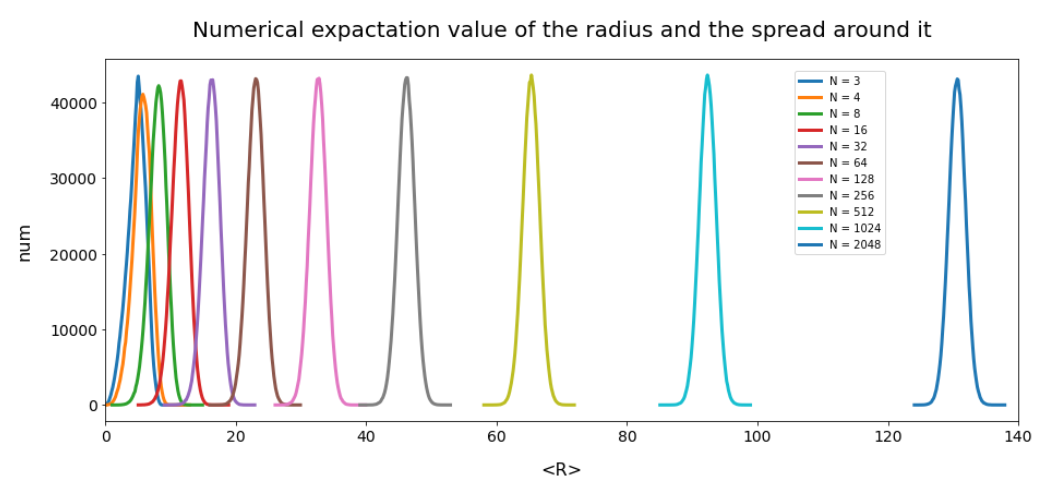
Note that one should be careful not to assume more than a point concentration in regions of a multi-dimensional spherical shell. Even within such a shell the created data points may avoid certain regions. I will give some arguments that support this point of view in the next post. But already now it has become very clear that a statistical distribution of vectors with constant probabilities of component values per dimension will not at all fill the latent space homogeneously.

Some better approximations for <R> and the relative standard deviation

The above formulas suffer from the fact that

\[ \sqrt{\lt R^{\,2} \gt} \: \gtrsim \: \lt R \gt
\]

is only a rough approximation which overestimates the real $lt; R > – value, which comes out of numerical simulations. The deviation rises sharply with a small number of dimensions. For a thorough discussion of how good the approximation is see the answer and links at the following discussion at stackexchange
https://stats.stackexchange.com/ questions/ 317095/ expectation-of-square-root-of-sum-of-independent-squared-uniform-random-variable

Below I give you a better approximation to < R >, which should be sufficient for most purposes and N ≥ 3:

\[ \lt R \gt \: \approx \: = \: b * \sqrt{ 1 /3 * N \,} * \sqrt{{1 \over {1 + {1 \over 4N} }} }
\]

This approximation can in turn be used to improve the ratio of the standard deviation to < N gt;:

\[ {1 \over {\left< R \right>} } * \sqrt{ \left< \, \left( \, R \, – \lt R \gt \, \right)^{2} \, \right> \,} \: \approx \: \sqrt{ 1 / (5N) \, } * {1 \over {1 + {1 \over 4N} }}
\]

Conclusion and outlook on the next post

In this post I have tried to fill a cube around the origin of a multi-dimensional orthogonal coordinate system with statistical points. I have assumed a constant probability density for each component of the respective vectors. A simple mathematical analysis leads to the somewhat surprising conclusion that the resulting data distribution concentrates in regions which are located within a multi-dimensional spherical shell. This shell becomes narrower and narrower with a rising number of dimensions N.

In the next post

Latent spaces – pitfalls of distributing points in multi dimensions – II – missing specific regions

I shall first prove the derived results and given approximations by numerical data. Then I will discuss what kind of regions, that a Neural Network might fill in its latent space, we will miss by such an approach.
 

Opensuse Leap 15.4 on a PC – III – fixing the order of multiple screens for SDDM and for Plasma, Gnome on Wayland

In the first post of this series I have covered the upgrade procedure of a Linux PC from Opensuse Leap 15.3 to Leap 15.4. In the second post I tested the system’s behavior for Plasma and Gnome on (X)Wayland. Which was surprisingly good.

Opensuse Leap 15.4 on a PC – I – Upgrade from Leap 15.3 – repositories, Nvidia, Vmware WS, KVM, Plasma widget deficits

Opensuse Leap 15.4 on a PC – II – Plasma, Gnome, flatpak, Libreoffice and others on (X)Wayland?

The upgrade to Leap 15.4 may come with an inconvenience on systems with multiple attached screens:

You may loose your preferred screen order.

This means that your mouse cursor may not move across your screens as you expect it for your desktop display manager or for your graphical desktop spanned over the number of available screens. And windows moved on the desktop across the right edge of a particular screen may appear on another screen physically positioned to the left of your current screen. Which is not really funny.

Actually, my upgrade to Leap 15.4 confronted me with a wrong screen order for both SDDM and my KDE Plasma desktop sessions. This happened on two of my systems – both equipped with Nvidia graphics cards. Regarding Plasma and Gnome on X11 I have previously often used the nvidia-settings application to fix the screen order and put related statements into the xorg.conf. But on (X)Wayland this is currently not an option. nvidia-settings simply lacks the required functionality there.

Some people recommend in such a case to switch cables between the available plugs at the graphics card. No need to do so. In the present post I show you how to get your screens into the required order again without moving their physical positions or putting their video cables into different plugs.

But I only describe the measures for the display manager SDDM and for KDE Plasma and Gnome on Wayland / X11. For other display managers and desktop environments other tools and steps may have to be applied. Below I use the term (X)Wayland when the methods apply both to a native Wayland session or a Xwayland setup.

Continue reading →

Autoencoders and latent space fragmentation – I – Encoder, Decoder, latent space

This series of posts is about a special kind of Artificial Neural Networks [ANNs] – namely so called Autoencoders [AEs] and their questionable creative abilities.

The series replaces two previous posts in this blog on a similar topic. My earlier posts were not wrong regarding the results of calculations presented there, but they contained premature conclusions. In this series I hope to perform a somewhat better analysis.

Abilities of Autoencoders and the question of a creative application of AEs

On the one hand side AEs can be trained to encode and compress object information. On the other hand side AEs can decode previously encoded information and reconstruct related original objects from the retrieved information.

A simple application of an AE, therefore, is the compression of image data and the reconstruction of images from compressed data. But, after a suitable adaption of the training process and its input data, we can also use AEs for other purposes. Examples are the denoising of disturbed images or the recoloring of grey images. In the latter cases the reconstructive properties of AEs play an important role.

An interesting question is: Can one utilize the reconstructive abilities of an AE for generative or creative purposes?

This post series will give an answer for the special case of images showing human faces. To say it clearly: I am talking about conventional AEs, not about Variational Autoencoders and neither about state of the art AEs based on transformer technology.

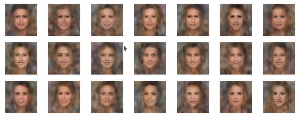
Most text books on Machine Learning [ML] would claim that at least Variational Autoencoders (instead of AEs) are required to create reasonable images of human faces … Well, to trigger a bit of your attention: Below you find some images of human faces created by standard Autoencoder – and NOT by a Variational Autoencoder.

I admit: These pictures are far from perfect, but at least they show clear features of human faces. Not exactly what we expect of a pure conventional Autoencoder fed with statistical input. I apologize for the bias towards female faces, but that is a “prejudice” of the AE caused by my chosen set of training data. And the lack of hairdo-details will later be commented on.

I promise: Analyzing the behavior of conventional AEs is still an interesting topic. Despite many and sophisticated modern alternatives for creative purposes. The reason is that we learn something about the way how an AE organizes the information which it gains during training.

Continue reading →

Opensuse Leap 15.4 on a PC – II – Plasma, Gnome, flatpak, Libreoffice and others on (X)Wayland?

In the last post of this series

Upgrade to Opensuse Leap 15.4 – I – a look at repositories, Nvidia, Vmware WS, KVM, Plasma widgets

we saw that an upgrade from Leap Opensuse 15.3 to Leap 15.4 is a relatively smooth operation. After the basic upgrade I wanted to look a bit at an interesting detail – namely (X)Wayland. And got surprised – positively and negatively. This post summarizes some of my experiences.

Nvidia and Wayland

For a long time it was almost impossible to use Wayland in combination with Nvidia and KDE. Which mostly was the fault of Nvidia. See an Heise article on this topic here. See also the experience of a Gnome user here – although I do not share his bad experience with a X11-based KDE Plasma on Nvidia. For years I have not seen a realistic chance for a productive use of Wayland on my PCs and laptops with Nvidia-cards. KDE PLasma did not work at all on Wayland. Also with Gnome I experienced terrible difficulties. But Nvidia has improved its support for Wayland significantly in 2022, starting with driver version 470. For Nvidia driver version 525 we would expect some stability.

Continue reading →

Opensuse Leap 15.4 on a PC – I – Upgrade from Leap 15.3 – repositories, Nvidia, Vmware WS, KVM, Plasma widget deficits

Today I upgraded a desktop PC with an Nvidia graphics card from Opensuse Leap 15.3 to Leap 15.4. I really must say: This was one of the smoothest upgrades I have ever experienced with Opensuse. However, there were again a few standard problems which had to be solved.

In this first post I summarize the upgrade steps and check the basic functionality of KDE/Plasma, VMware Workstation and KVM. I will also comment on some deficits of Plasma widgets for system monitoring.

In a second posts I summarize a brief test of Xwayland. A third post will discuss how to define a screen order for situations where multiple screens are attached to your PC. A brief fourth post will discuss PHP8 and Apache2 settings. We will also check that Eclipse works for PHP and Python/PyDeV. I will also verify the functionality of Python3 (3.9/3.10), Tensorflow2 and Jupyter after the upgrade. A last post provides solutions for multi-soundcard setups with Pulseaudio and pavucontrol.

PC components – and major SW

My PC has two major raid-systems – one with multiple SSDs (at an Intel controller, set up and controlled with the help of Linux mdraid) and one with HDs (3ware controller). The raid systems host LVM volumes and ordinary partitions. The graphics card is a relatively old Nvidia card. Two sound cards (X-Fi, Xonar D2X) are used in parallel. My standard desktop is KDE/Plasma scaled over 3 screens. For virtualization of Windows 10 VMware WS 16 is used. Virtualized Linux systems, however, run on KVM/qemu with virtual spice screens. PHP development is done with the help of Eclipse and a local Apache server. Machine Learning development is done with Python3 (3.9), PyDEV (Eclipse), Tensorflow2/Keras, Juypter.

Upgrade procedure

Regarding the basic upgrade procedure you can adapt steps which I have extensively described for a laptop here. You can just ignore any steps regarding an Optimus based combination of graphics cards.

List of steps

  • Step 1:Make backups! Especially of the LVM volumes or partitions which host your root filesystem and your /home-directory.
  • Step 2: Check your repositories! Save a list of your active ones and their URLs. Reason: Some repository paths below “download.opensuse.org” have changed and you need to include these repos again into zypper. Below I give some information on repositories which directly can be upgraded with the help of ${releasever}.
  • Step 3: Update your current RPMs.
  • Step 4: In a terminal window:
    mytux:~ # zypper refresh
    mytux:~ # zypper update

    Then restart your system and verify that it is working.

  • Step 5: In a terminal window change repo URLs to include ${releasever}
    mytux:~ # sed -i 's/15.3/${releasever}/g' /etc/zypp/repos.d/*.repo
    mytux:~ # sed -i 's/$releasever/${releasever}/g' /etc/zypp/repos.d/*.repo
    
  • Step 6: In a terminal window test a refesh for the Leap 15.4 repos:
    mytux:~ # zypper --releasever=15.4 refresh
    

    If there are problems analyze the reason and eliminate those repositories whose URL have changed. Re-check the success of the refresh.

  • Step 7: In a terminal window download the new RPMs
    mytux:~ #  zypper --releasever=15.4 dup --download-only --allow-vendor-change
    
  • Step 8: Close the graphical desktop and switch to a TTY (Ctrl-Alt-F1). Stop the display server and then upgrade
    mytux:~ # init 3 
    mytux:~ # zypper --no-refresh --releasever=15.4 dup --allow-vendor-change
    
  • Step 9: Pray and reboot to your upgraded Opensuse Leap 15.4

With selected repositories discussed below all these steps could be performed without major problems.

My good news are: There were no problems regarding drivers for the Nvidia card (see below), the raid controllers and my multiple Raid 5 and Raid 10 setups with LVM groups and LVM volumes. No problem was seen regarding Grub2 and systemd.

Which repositories can be directly upgraded via ${releasever}?

Central repositories for the upgrade are

https://download.opensuse.org/update/leap/15.4/oss/
http://download.opensuse.org/update/leap/15.4/backports/
http://download.opensuse.org/update/leap/15.4/sle/

Their 15.3 precedessors must be active. You need to refresh them and replace the “15.3” in their addresses by “${releasever}”. See my post named above for the required steps. Aside of the central repositories I kept some others active during the upgrade process (with ${releasever}). Worth to name:

https://download.opensuse.org/repositories/LibreOffice:/7.5/openSUSE_Leap_15.4/
https://download.nvidia.com/opensuse/leap/15.4
https://developer.download.nvidia.com/compute/cuda/repos/opensuse15/x86_64
https://ftp.fau.de/packman/suse/openSUSE_Leap_15.4/
https://download.opensuse.org/repositories/mozilla/openSUSE_Leap_15.4/
https://download.opensuse.org/repositories/devel:/languages:/php/openSUSE_Leap_15.4/

These repositories cause no problems as their URLs for 15.3 and 15.4 only show a difference regarding their release version but not their position in the URL-tree below “download.opensuse.org”. However, some other repositories, like those for X2GO, graphics, network, security have changed their position in the URL-resource-tree and must be reconfigured after the upgrade – e.g with the help of YaST or zypper.

Nvidia driver and the new kernel

On Leap 15.3 I had used the latest Nvidia driver from the usual Nvidia community repository

download.nvidia.com/opensuse/leap/${releasever}

The active RPM was replaced by the one from the Leap 15.4 repo during upgrade resulting in the RPM “nvidia-compute-G06”, version 525.89.02-lp154.5.1. Both the transition to the respective Nvidia kernel module for the new kernel 5.14.21 and the module’s inclusion in the system’s startup procedures by dracut went without any faults.

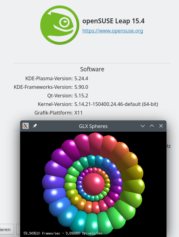
The upgraded system directly started into a SDDM login screen. There as a mess regarding my screen order (see a forthcoming post), but this did not hinder a proper login. Afterward KDE/Plasma (in combination with Xorg) started on the three screens attached to my PC. Though I feel that the startup of KDE/Plasma for Xorg takes a more time than on Leap 15.3. But I could see no major problems. GLX applications were running as expected.

VMware Workstation WS 16.2.5 works!

As I already saw with a Leap 15.4 installation on a laptop: VMware WS 16.2.5 works with Leap 15.4 and Kernel 5.14.21. Actually, already version WS 16.2.3 is compatible.

KVM/Qemu works with installed virtual systems!

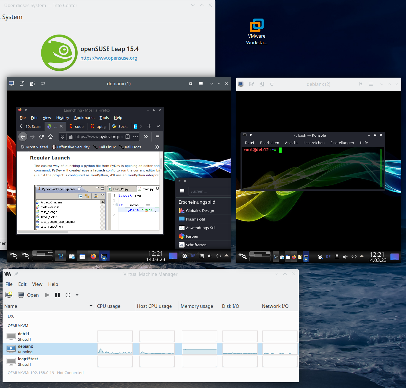
The transition of KV, qemu und libvitrtd went smoothly. virt-manager works and starts installed virtual systems as expected:

KDE – plasma-systemmonitor and respective widgets do not show information on Nvidia graphics card and not all information on network cards

At least on my system with KDE Plasma 5.24.4 (KDE Framework 5.90) I saw major deficits regarding apps and widgets which should monitor the status of system resources:

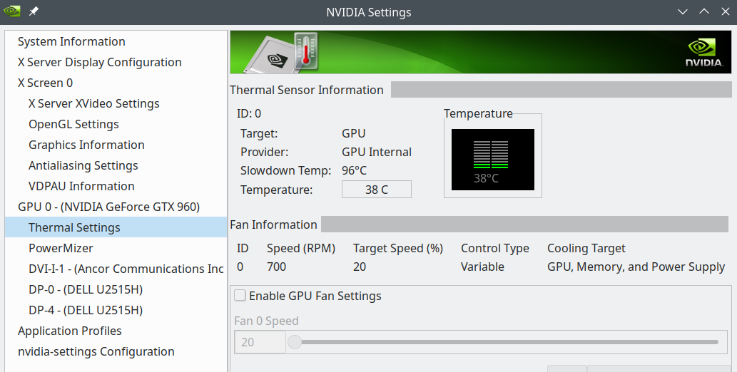
  • Problem 1 – no information about the status of the Nvidia GPU: Neither the application “systemmonitor” nor related widgets can deliver information about the status of the NVidia card (temperature, VRAM usage, fan) – with the (useless) exception of the type of the card. See th eimage in the next section. (Note that lm_sensors do not help in this case as the HW sensors did not detect the Nvidia card either.)
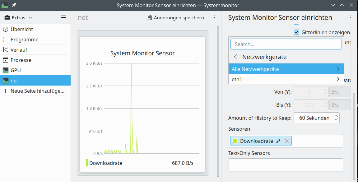
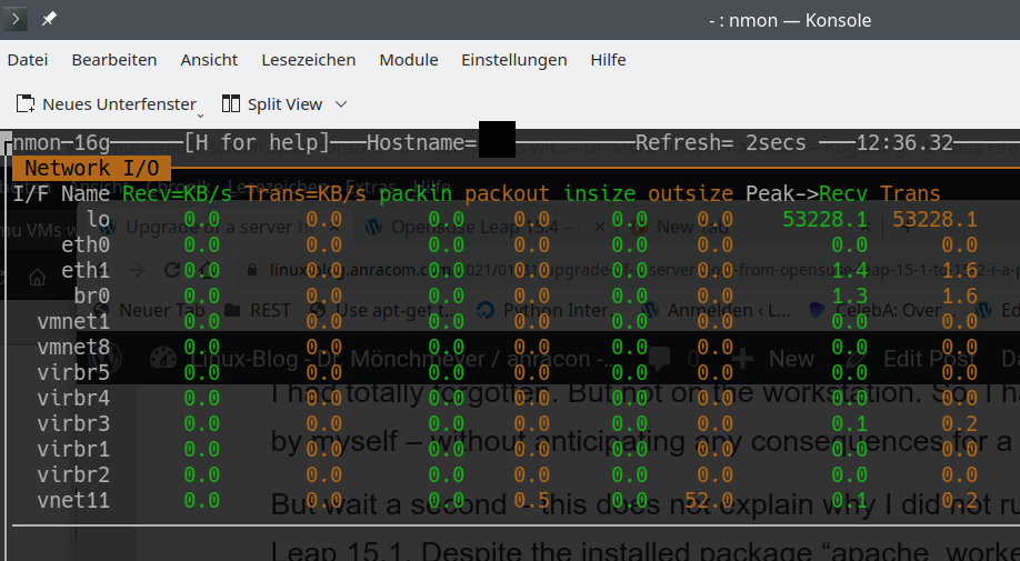
  • Problem 2 – no information about virtual network devices: In addition the KDE/Plasma widgets were not able to display all data for network interfaces correctly. E.g. interfaces like lo, bridges and other virtual devices were not even listed. And thus on a more complex configuration with virtualization you will not see your IP addresses with the Plasma-tools.

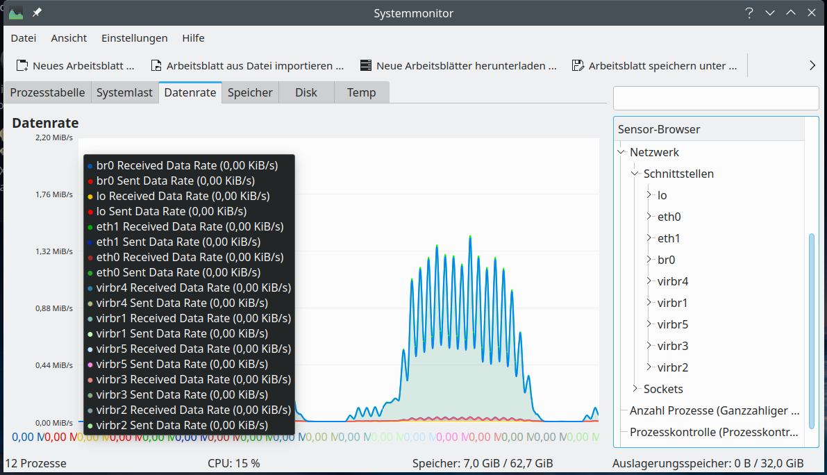
Regarding the second point: The image below shows that the dialog to set up network monitoring only offers to select an active physical device, in my case eth1. But no virtual devices which are available, too.

And here the devices nmon lists up:

These are clearly Plasma problems as other basic Linux and desktop applications perform much better for the named resources. Someone who works with Machine Learning and with virtualized Linux installations needs to watch the GPU (fans and temperature) and traffic across network devices – virtualized or real. This does not seem to be something we can get from fancy KDE/Plasma widgets today. So, we have to look out for alternatives.

Alternatives to watch the temperature of Nvidia GPUs

One prominent example which covers more than the present KDE widgets for system monitoring is the good old “gkrellm“. I love it, really! Compact, with a lot of already integrated default “sensors” and compatible to lm_sensors! And it delivers me the GPU temperature.

Another desktop tool with a somewhat old fashioned presentation of graphics is psensor. You can get a binary for Leap 15.4 from the “home”-repository of plasmaaregataos.

https://download.opensuse.org/repositories/home:/plasmaregataos/15.4/

Interesting, how much this tool finds out about the Nvidia card (where Plasma tools fail totally).

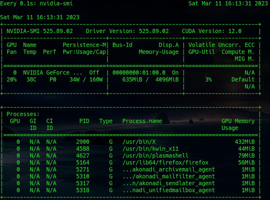
And then we have, of course, Nvidia’s own tools: nvidia-settings (graphical) and nvidia-smi (ASCII):

Note that the command to periodically update the nvidia-smi information is:

watch -n0.1 nvidia-smi

Alternatives to watch the data traffic across all network devices – real and virtual

Once again I have to name gkrellm. It provides a lot of information on real and virtual network interface.

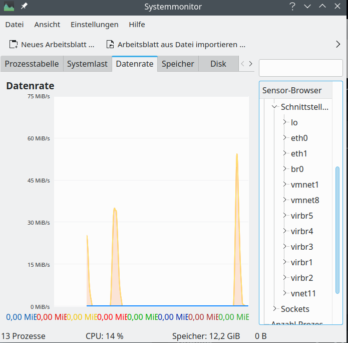
Regarding a graphical information on virtual network interfaces we can also use a relatively old KDE tool, namely ksysguard. Besides real network interfaces it detects bridges and KVM or Vmware based virtual devices and tracks their load.

Hint for those who worry about the discrepancy with the screenshot for nmon above: Some devices which nmon showed were not available at the time of the screenshot of ksysguard as certain KVM virtual machines and networks were not yet started. Later ksysguard detects other devices, too:

Based on ncurses you can also use the network part of “nmon” to get information on transfer rates across all defined network interfaces. If you need to go more into details a very good ASCII tool is “iptraf-ng“. “iftop” is also cool, but to watch multiple interfaces in parallel you have to use the command “iftop -i” on multiple terminal windows.

So, dear Plasma developers: When can we expect a fancy Plasma applications or widgets which reproduce and combine the “sensoric” abilities of gkrellm, psensor, ksysguard and iptraf-ng?

Conclusion

The upgrade from Leap 15.3 to Leap 15.4 posed no major problems on my PC. A relatively old VMware WS 16.2.x still worked and there were no problems regarding KVM/qemu. The new Nvidia driver could be compiled without any problems for the new kernel during upgrade and was directly integrated into the system by dracut. The new KDE/Plasma version started without problems on Xorg. Deficits of Plasma widgets for monitoring system devices were obvious; but this is not something we can blame Opensuse for.

In the next post of this series

Opensuse Leap 15.4 on a PC – II – Plasma, Gnome, flatpak, Libreoffice and others on (X)Wayland?

I will have a look at KDE/Plasma started on Xwayland.

Happy working with Opensuse Leap 15.4 and stay tuned …