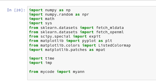
I continue with my series on a Python program for coding small “Multilayer Perceptrons” [MLPs].
A simple program for an ANN to cover the Mnist dataset – VII – EBP related topics and obstacles
A simple program for an ANN to cover the Mnist dataset – VI – the math behind the „error back-propagation“
A simple program for an ANN to cover the Mnist dataset – V – coding the loss function
A simple program for an ANN to cover the Mnist dataset – IV – the concept of a cost or loss function
A simple program for an ANN to cover the Mnist dataset – III – forward propagation
A simple program for an ANN to cover the Mnist dataset – II – initial random weight values
A simple program for an ANN to cover the Mnist dataset – I – a starting point
After all the theoretical considerations of the last two articles we now start coding again. Our objective is to extend our methods for training the MLP on the MNIST dataset by methods which perform the “error back propagation” and the correction of the weights. The mathematical prescriptions were derived in the following PDF:
My PDF on “The math behind EBP”
When you study the new code fragments below remember a few things:
We are prepared to use mini-batches. Therefore, the cost functions will be calculated over the data records of each batch and all the matrix operations for back propagation will cover all batch-records in parallel. Training means to loop over epochs and mini-batches – in pseudo-code:
- Loop over epochs
- adjust learning rate,
- check for convergence criteria,
- Shuffle all data records in the test data set and build new mini-batches
- Loop over mini-batches
- Perform forward propagation for all records of the mini-batch
- calculate and save the total cost value for each mini-batch
- calculate and save an averaged error on the output layer for each mini-batch
- perform error backward propagation on all records of the mini-batch to get the gradient of the cost function with respect to all weights
- adjust all weights on all layers
As discussed in the last article: The cost hyperplane changes a bit with each mini-batch. If there is a good mixture of records in a batch then the form of its specific cost hyperplane will (hopefully) resemble the form of an overall cost hyperplane, but it will not be the same. By the second step in the outer loop we want to avoid that the same data records always get an influence on the gradients at the same position in the correction procedure. Both statistical elements help a bit to overcome dominant records and a non-equal distribution of test records. If we had only pictures for number 3 at the end of our MNIST data set we
may start learning “3” representations very well, but not other numbers. Statistical variation also helps to avoid side minima on the overall cost hyperplane for all data records of the test set.
We shall implement the second step and third step in the epoch loop in the next article – when we are sure that the training algorithm works as expected. So, at the moment we will stop our training only after a given number of epochs.
More input parameters
In the first articles we had build an __init__()-method to parameterize a training run. We have to include three more parameters to control the backward propagation.
learn_rate = 0.001, # the learning rate (often called epsilon in textbooks)
decrease_const = 0.00001, # a factor for decreasing the learning rate with epochs
mom_rate = 0.0005, # a factor for momentum learning
The first parameter controls by how much we change weights with the help of gradient values. See formula (93) in the PDF of article VI (you find the Link to the latest version in the last section of this article). The second parameter will give us an option to decrease the learning rate with the number of training epochs. Note that a constant decrease rate only makes sense, if we can be relatively sure that we do not end up in a side minimum of the cost function.
The third parameter is interesting: It will allow us to mix the presently calculated weight correction with the correction term from the last step. So to say: We extend the “momentum” of the last correction into the next correction. This helps us not to follow indicated direction changes on the cost hyperplanes too fast.
Some hygienic measures regarding variables
In the already written parts of the code we have used a prefix “ay_” for all variables which represent some vector or array like structure – including Python lists and Numpy arrays. For back propagation coding it will be more important to distinguish between lists and arrays. So, I changed the variable prefix for some important Python lists from “ay_” to “li_”. (I shall do it for all lists used in a further version). In addition I have changed the prefix for Python ranges to “rg_”. These changes will affect the contents and the interface of some methods. You will notice when we come to these methods.
The changed __input__()-method
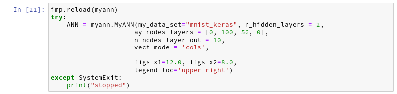
Our modified __init__() function now looks like this:
def __init__(self,
my_data_set = "mnist",
n_hidden_layers = 1,
ay_nodes_layers = [0, 100, 0], # array which should have as much elements as n_hidden + 2
n_nodes_layer_out = 10, # expected number of nodes in output layer
my_activation_function = "sigmoid",
my_out_function = "sigmoid",
my_loss_function = "LogLoss",
n_size_mini_batch = 50, # number of data elements in a mini-batch
n_epochs = 1,
n_max_batches = -1, # number of mini-batches to use during epochs - > 0 only for testing
# a negative value uses all mini-batches
lambda2_reg = 0.1, # factor for quadratic regularization term
lambda1_reg = 0.0, # factor for linear regularization term
vect_mode = 'cols',
learn_rate = 0.001, # the learning rate (often called epsilon in textbooks)
decrease_const = 0.00001, # a factor for decreasing the learning rate with epochs
mom_rate
= 0.0005, # a factor for momentum learning
figs_x1=12.0, figs_x2=8.0,
legend_loc='upper right',
b_print_test_data = True
):
'''
Initialization of MyANN
Input:
data_set: type of dataset; so far only the "mnist", "mnist_784" datsets are known
We use this information to prepare the input data and learn about the feature dimension.
This info is used in preparing the size of the input layer.
n_hidden_layers = number of hidden layers => between input layer 0 and output layer n
ay_nodes_layers = [0, 100, 0 ] : We set the number of nodes in input layer_0 and the output_layer to zero
Will be set to real number afterwards by infos from the input dataset.
All other numbers are used for the node numbers of the hidden layers.
n_nodes_out_layer = expected number of nodes in the output layer (is checked);
this number corresponds to the number of categories NC = number of labels to be distinguished
my_activation_function : name of the activation function to use
my_out_function : name of the "activation" function of the last layer which produces the output values
my_loss_function : name of the "cost" or "loss" function used for optimization
n_size_mini_batch : Number of elements/samples in a mini-batch of training data
The number of mini-batches will be calculated from this
n_epochs : number of epochs to calculate during training
n_max_batches : > 0: maximum of mini-batches to use during training
< 0: use all mini-batches
lambda_reg2: The factor for the quadartic regularization term
lambda_reg1: The factor for the linear regularization term
vect_mode: Are 1-dim data arrays (vctors) ordered by columns or rows ?
learn rate : Learning rate - definies by how much we correct weights in the indicated direction of the gradient on the cost hyperplane.
decrease_const: Controls a systematic decrease of the learning rate with epoch number
mom_const: Momentum rate. Controls a mixture of the last with the present weight corrections (momentum learning)
figs_x1=12.0, figs_x2=8.0 : Standard sizing of plots ,
legend_loc='upper right': Position of legends in the plots
b_print_test_data: Boolean variable to control the print out of some tests data
'''
# Array (Python list) of known input data sets
self._input_data_sets = ["mnist", "mnist_784", "mnist_keras"]
self._my_data_set = my_data_set
# X, y, X_train, y_train, X_test, y_test
# will be set by analyze_input_data
# X: Input array (2D) - at present status of MNIST image data, only.
# y: result (=classification data) [digits represent categories in the case of Mnist]
self._X = None
self._X_train = None
self._X_test = None
self._y = None
self._y_train = None
self._y_test = None
# relevant dimensions
# from input data information; will be set in handle_input_data()
self._dim_sets = 0
self._dim_features = 0
self._n_labels = 0 # number of unique labels - will be extracted from y-data
# Img sizes
self._dim_img = 0 # should be sqrt(dim_features) - we assume square like images
self._img_h = 0
self._img_w = 0
# Layers
# ------
# number of hidden layers
self._n_hidden_layers = n_hidden_layers
# Number of total layers
self._n_total_layers = 2 + self._n_hidden_layers
# Nodes for hidden layers
self._ay_nodes_layers = np.array(ay_nodes_layers)
# Number of nodes in output layer - will be checked against information from target arrays
self._n_nodes_layer_out = n_nodes_layer_out
# Weights
# --------
# empty List for all weight-matrices for all layer-connections
# Numbering :
# w[0] contains the weight matrix which connects layer 0 (input layer ) to hidden layer 1
# w[1] contains the weight matrix which connects layer 1 (input layer ) to (hidden?) layer 2
self._li_w = []
# Arrays for encoded output labels - will be set in _encode_all_mnist_labels()
# -------------------------------
self._ay_onehot = None
self._ay_oneval = None
# Known Randomizer methods ( 0: np.random.randint, 1: np.random.uniform )
# ------------------
self.__ay_known_randomizers = [0, 1]
# Types of activation functions and output functions
# ------------------
self.__ay_activation_functions = ["sigmoid"] # later also relu
self.__ay_output_functions = ["sigmoid"] # later also softmax
# Types of cost functions
# ------------------
self.__ay_loss_functions = ["LogLoss", "MSE" ] # later also othr types of cost/loss functions
# the following dictionaries will be used for indirect function calls
self.__d_activation_funcs = {
'sigmoid': self._sigmoid,
'relu': self._relu
}
self.__d_output_funcs = {
'sigmoid': self._sigmoid,
'softmax': self._softmax
}
self.__d_loss_funcs = {
'LogLoss': self._loss_LogLoss,
'MSE': self._loss_MSE
}
# Derivative functions
self.__d_D_activation_funcs = {
'sigmoid': self._D_sigmoid,
'relu': self._D_relu
}
self.__d_D_output_funcs = {
'sigmoid': self._D_sigmoid,
'softmax': self._D_softmax
}
self.__d_D_loss_funcs = {
'LogLoss': self._D_loss_LogLoss,
'MSE': self._D_loss_MSE
}
# The following variables will later be set by _check_and set_activation_and_out_functions()
self._my_act_func = my_activation_function
self._my_out_func = my_out_function
self._my_loss_func = my_loss_function
self._act_func = None
self._out_func = None
self._loss_func = None
# number of data samples in a mini-batch
self._n_size_mini_batch = n_size_mini_batch
self._n_mini_batches = None # will be determined by _get_number_of_mini_batches()
# maximum number of epochs - we set this number to an assumed maximum
# - as we shall build a backup and reload functionality for training, this should not be a major problem
self._n_epochs = n_epochs
# maximum number of batches to handle ( if < 0 => all!)
self._n_max_batches = n_max_batches
# actual number of batches
self._n_batches = None
# regularization parameters
self._lambda2_reg = lambda2_reg
self._
lambda1_reg = lambda1_reg
# parameter for momentum learning
self._learn_rate = learn_rate
self._decrease_const = decrease_const
self._mom_rate = mom_rate
self._li_mom = [None] * self._n_total_layers
# book-keeping for epochs and mini-batches
# -------------------------------
# range for epochs - will be set by _prepare-epochs_and_batches()
self._rg_idx_epochs = None
# range for mini-batches
self._rg_idx_batches = None
# dimension of the numpy arrays for book-keeping - will be set in _prepare_epochs_and_batches()
self._shape_epochs_batches = None # (n_epochs, n_batches, 1)
# list for error values at outermost layer for minibatches and epochs during training
# we use a numpy array here because we can redimension it
self._ay_theta = None
# list for cost values of mini-batches during training
# The list will later be split into sections for epochs
self._ay_costs = None
# Data elements for back propagation
# ----------------------------------
# 2-dim array of partial derivatives of the elements of an additive cost function
# The derivative is taken with respect to the output results a_j = ay_ANN_out[j]
# The array dimensions account for nodes and sampls of a mini_batch. The array will be set in function
# self._initiate_bw_propagation()
self._ay_delta_out_batch = None
# parameter to allow printing of some test data
self._b_print_test_data = b_print_test_data
# Plot handling
# --------------
# Alternatives to resize plots
# 1: just resize figure 2: resize plus create subplots() [figure + axes]
self._plot_resize_alternative = 1
# Plot-sizing
self._figs_x1 = figs_x1
self._figs_x2 = figs_x2
self._fig = None
self._ax = None
# alternative 2 does resizing and (!) subplots()
self.initiate_and_resize_plot(self._plot_resize_alternative)
# ***********
# operations
# ***********
# check and handle input data
self._handle_input_data()
# set the ANN structure
self._set_ANN_structure()
# Prepare epoch and batch-handling - sets ranges, limits num of mini-batches and initializes book-keeping arrays
self._rg_idx_epochs, self._rg_idx_batches = self._prepare_epochs_and_batches()
# perform training
start_c = time.perf_counter()
self._fit(b_print=True, b_measure_batch_time=False)
end_c = time.perf_counter()
print('\n\n ------')
print('Total training Time_CPU: ', end_c - start_c)
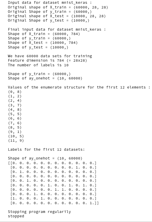
print("\nStopping program regularily")
sys.exit()
The extended method _set_ANN_structure()
I do not change method “_handle_input_data()”. However, I extend method “def _set_ANN_structure()” by a statement to initialize a list with momentum matrices for all layers.
    '''-- Method to set ANN structure --'''
    def _set_ANN_structure(self):
        # check consistency of the node-number list with the number of hidden layers (n_hidden)
        self._check_layer_and_node_numbers()
        # set node numbers for the input layer and the output layer
        self._set_nodes_for_input_output_layers()
        self._show_node_numbers()

        # create the weight matrix between input and first hidden layer
        self._create_WM_Input()
        # create weight matrices between the
hidden layers and between tha last hidden and the output layer
        self._create_WM_Hidden()

        # initialize momentum differences
        self._create_momentum_matrices()
        #print("\nLength of li_mom = ", str(len(self._li_mom)))

        # check and set activation functions
        self._check_and_set_activation_and_out_functions()
        self._check_and_set_loss_function()

        return None
The following box shows the changed functions _create_WM_Input(), _create_WM_Hidden() and the new function _create_momentum_matrices():
    '''-- Method to create the weight matrix between L0/L1 --'''
    def _create_WM_Input(self):
        '''
        Method to create the input layer
        The dimension will be taken from the structure of the input data
        We need to fill self._w[0] with a matrix for conections of all nodes in L0 with all nodes in L1
        We fill the matrix with random numbers between [-1, 1]
        '''
        # the num_nodes of layer 0 should already include the bias node
        num_nodes_layer_0 = self._ay_nodes_layers[0]
        num_nodes_with_bias_layer_0 = num_nodes_layer_0 + 1
        num_nodes_layer_1 = self._ay_nodes_layers[1]

        # fill the matrix with random values
        #rand_low  = -1.0
        #rand_high = 1.0
        rand_low  = -0.5
        rand_high = 0.5
        rand_size = num_nodes_layer_1 * (num_nodes_with_bias_layer_0)

        randomizer = 1 # method np.random.uniform

        w0 = self._create_vector_with_random_values(rand_low, rand_high, rand_size, randomizer)
        w0 = w0.reshape(num_nodes_layer_1, num_nodes_with_bias_layer_0)

        # put the weight matrix into array of matrices
        self._li_w.append(w0)
        print("\nShape of weight matrix between layers 0 and 1 " + str(self._li_w[0].shape))

#
    '''-- Method to create the weight-matrices for hidden layers--'''
    def _create_WM_Hidden(self):
        '''
        Method to create the weights of the hidden layers, i.e. between [L1, L2] and so on ... [L_n, L_out]
        We fill the matrix with random numbers between [-1, 1]
        '''

        # The "+1" is required due to range properties !
        rg_hidden_layers = range(1, self._n_hidden_layers + 1, 1)

        # for random operation
        rand_low  = -1.0
        rand_high = 1.0

        for i in rg_hidden_layers:
            print ("Creating weight matrix for layer " + str(i) + " to layer " + str(i+1) )

            num_nodes_layer = self._ay_nodes_layers[i]
            num_nodes_with_bias_layer = num_nodes_layer + 1

            # the number of the next layer is taken without the bias node!
            num_nodes_layer_next = self._ay_nodes_layers[i+1]

            # assign random values
            rand_size = num_nodes_layer_next * num_nodes_with_bias_layer

            randomizer = 1 # np.random.uniform

            w_i_next = self._create_vector_with_random_values(rand_low, rand_high, rand_size, randomizer)
            w_i_next = w_i_next.reshape(num_nodes_layer_next, num_nodes_with_bias_layer)

            # put the weight matrix into our array of matrices
            self._li_w.append(w_i_next)
            print("Shape of weight matrix between layers " + str(i) + " and " + str(i+1) + " = " + str(self._li_w[i].shape))
#
    '''-- Method to create and initialize matrices for momentum learning (differences) '''
    def _create_momentum_matrices(self):
        rg_layers = range(0, self._n_total_layers - 1)
        for i in rg_layers:
r
            self._li_mom[i] = np.zeros(self._li_w[i].shape)
            #print("shape of li_mom[" + str(i) + "] = ", self._li_mom[i].shape)
The modified functions _fit() and _handle_mini_batch()
The _fit()-function is modified to include a systematic decrease of the learning rate.
    ''' -- Method to set the number of batches based on given batch size -- '''
    def _fit(self, b_print = False, b_measure_batch_time = False):

        rg_idx_epochs  = self._rg_idx_epochs
        rg_idx_batches = self._rg_idx_batches
        if (b_print):
            print("\nnumber of epochs = " + str(len(rg_idx_epochs)))
            print("max number of batches = " + str(len(rg_idx_batches)))

        # loop over epochs
        for idxe in rg_idx_epochs:
            if (b_print):
                print("\n ---------")
                print("\nStarting epoch " + str(idxe+1))

                self._learn_rate /= (1.0 + self._decrease_const * idxe)

            # loop over mini-batches
            for idxb in rg_idx_batches:
                if (b_print):
                    print("\n ---------")
                    print("\nDealing with mini-batch " + str(idxb+1))
                if b_measure_batch_time:
                    start_0 = time.perf_counter()
                # deal with a mini-batch
                self._handle_mini_batch(num_batch = idxb, num_epoch=idxe, b_print_y_vals = False, b_print = False)
                if b_measure_batch_time:
                    end_0 = time.perf_counter()
                    print('Time_CPU for batch ' + str(idxb+1), end_0 - start_0)

                #if idxb == 100:
                #    sys.exit()

        return None
Note that the number of epochs is determined by an external parameter as an upper limit of the range “rg_idx_epochs”.
Method “_handle_mini_batch()” requires several changes: First we define lists which are required to save matrix data of the backward propagation. And, of course, we call a method to perform the BW propagation (see step 6 in the code). Some statements print shapes, if required. At step 7 of the code we correct the weights by using the learning rate and the calculated gradient of the loss function.
Note, that we mix the correction evaluated at the last batch-record with the correction evaluated for the present record! This corresponds to a simple form of momentum learning. We then have to save the present correction values, of course. Note that the list for momentum correction “li_mom” is, therefore, not deleted at the end of a mini-batch treatment !
In addition to saving the total costs per mini-batch we now also save a mean error at the output level. The average is done by the help of Numpy’s function numpy.average() for matrices. Remember, we build the average over errors at all output nodes and all records of the mini-batch.
    ''' -- Method to deal with a batch -- '''
    def _handle_mini_batch(self, num_batch = 0, num_epoch = 0, b_print_y_vals = False, b_print = False, b_keep_bw_matrices = True):
        '''
        For each batch we keep the input data array Z and the output data A (output of activation function!)
        for all layers in Python lists
        We can use this as input variables in function calls - mutable variables are handled by reference values !
        We receive the A and Z data from propagation functions and proceed them to cost and gradient calculation functions

        As an initial step we define the Python lists li_Z_
in_layer and li_A_out_layer
        and fill in the first input elements for layer L0

        Forward propagation:
        --------------------
        li_Z_in_layer : List of layer-related 2-dim matrices for input values z at each node (rows) and all batch-samples (cols).
        li_A_out_layer: List of layer-related 2-dim matrices for output alues z at each node (rows) and all batch-samples (cols).
                        The output is created by Phi(z), where Phi represents an activation or output function

        Note that the matrices in ay_A_out will be permanently extended by a row (over all samples)
        to account for a bias node of each inner layer. This happens during FW propagation.

        Note that the matrices ay_Z_in will be temporarily extended by a row (over all samples)
        to account for a bias node of each inner layer. This happens during BW propagation.

        Backward propagation:
        --------------------
        li_delta_out:  Startup matrix for _out_delta-values at the outermost layer
        li_grad_layer: List of layer-related matrices with gradient values for the correction of the weights

        Depending on parameter "b_keep_bw_matrices" we keep
            - a list of layer-related matrices D with values for the derivatives of the act./output functions
            - a list of layer-related matrices for the back propagated delta-values
        in lists during back propagation. This can support error analysis.

        All matrices in the lists are 2 dimensional with dimensions for nodes (rows) and training samples (cols)
        All these lists be deleted at the end of the function to accelerate garbadge handling

        Input parameters:
        ----------------
        num_epoch:     Number of present epoch
        num_batch:    Number of present mini-batch
        '''
        # Layer-related lists to be filled with 2-dim Numpy matrices during FW propagation
        # ********************************************************************************
        li_Z_in_layer  = [None] * self._n_total_layers # List of matrices with z-input values for each layer; filled during FW-propagation
        li_A_out_layer = li_Z_in_layer.copy()          # List of matrices with results of activation/output-functions for each layer; filled during FW-propagation
        li_delta_out   = li_Z_in_layer.copy()          # Matrix with out_delta-values at the outermost layer
        li_delta_layer = li_Z_in_layer.copy()          # List of the matrices for the BW propagated delta values
        li_D_layer     = li_Z_in_layer.copy()          # List of the derivative matrices D containing partial derivatives of the activation/ouput functions
        li_grad_layer  = li_Z_in_layer.copy()          # List of the matrices with gradient values for weight corrections

        if b_print:
            len_lists = len(li_A_out_layer)
            print("\nnum_epoch = ", num_epoch, "  num_batch = ", num_batch )
            print("\nhandle_mini_batch(): length of lists = ", len_lists)
            self._info_point_print("handle_mini_batch: point 1")

        # Print some infos
        # ****************
        if b_print:
            self._print_batch_infos()
            self._info_point_print("handle_mini_batch: point 2")

        # Major steps for the mini-batch during one epoch iteration
        # **********************************************************

        # Step 0: List of indices for data records in the present mini-batch
        # ******
        ay_idx_batch = self._ay_mini_batches[num_batch]

        # Step 1: Special preparation of the Z-input to the MLP's input Layer L0
        # ******
        # Layer L0: Fill in the input vector for the ANN's input layer L0
        li_
Z_in_layer[0] = self._X_train[ay_idx_batch] # numpy arrays can be indexed by an array of integers
        if b_print:
            print("\nPropagation : Shape of X_in = li_Z_in_layer = ", li_Z_in_layer[0].shape)
            #print("\nidx, expected y_value of Layer L0-input :")
            #for idx in self._ay_mini_batches[num_batch]:
            #    print(str(idx) + ', ' + str(self._y_train[idx]) )
            self._info_point_print("handle_mini_batch: point 3")

        # Step 2: Layer L0: We need to transpose the data of the input layer
        # *******
        ay_Z_in_0T       = li_Z_in_layer[0].T
        li_Z_in_layer[0] = ay_Z_in_0T
        if b_print:
            print("\nPropagation : Shape of transposed X_in = li_Z_in_layer = ", li_Z_in_layer[0].shape)
            self._info_point_print("handle_mini_batch: point 4")

        # Step 3: Call forward propagation method for the present mini-batch of training records
        # *******
        # this function will fill the ay_Z_in- and ay_A_out-lists with matrices per layer
        self._fw_propagation(li_Z_in = li_Z_in_layer, li_A_out = li_A_out_layer, b_print = b_print)

        if b_print:
            ilayer = range(0, self._n_total_layers)
            print("\n ---- ")
            print("\nAfter propagation through all " + str(self._n_total_layers) + " layers: ")
            for il in ilayer:
                print("Shape of Z_in of layer L" + str(il) + " = " + str(li_Z_in_layer[il].shape))
                print("Shape of A_out of layer L" + str(il) + " = " + str(li_A_out_layer[il].shape))
                if il < self._n_total_layers-1:
                    print("Shape of W of layer L" + str(il) + " = " + str(self._li_w[il].shape))
                    print("Shape of Mom of layer L" + str(il) + " = " + str(self._li_mom[il].shape))
            self._info_point_print("handle_mini_batch: point 5")


        # Step 4: Cost calculation for the mini-batch
        # ********
        ay_y_enc = self._ay_onehot[:, ay_idx_batch]
        ay_ANN_out = li_A_out_layer[self._n_total_layers-1]
        # print("Shape of ay_ANN_out = " + str(ay_ANN_out.shape))

        total_costs_batch = self._calculate_loss_for_batch(ay_y_enc, ay_ANN_out, b_print = False)
        # we add the present cost value to the numpy array
        self._ay_costs[num_epoch, num_batch] = total_costs_batch
        if b_print:
            print("\n total costs of mini_batch = ", self._ay_costs[num_epoch, num_batch])
            self._info_point_print("handle_mini_batch: point 6")
        print("\n total costs of mini_batch = ", self._ay_costs[num_epoch, num_batch])

        # Step 5: Avg-error for later plotting
        # ********
        # mean "error" values - averaged over all nodes at outermost layer and all data sets of a mini-batch
        ay_theta_out = ay_y_enc - ay_ANN_out
        if (b_print):
            print("Shape of ay_theta_out = " + str(ay_theta_out.shape))
        ay_theta_avg = np.average(np.abs(ay_theta_out))
        self._ay_theta[num_epoch, num_batch] = ay_theta_avg

        if b_print:
            print("\navg total error of mini_batch = ", self._ay_theta[num_epoch, num_batch])
            self._info_point_print("handle_mini_batch: point 7")
        print("avg total error of mini_batch = ", self._ay_theta[num_epoch, num_batch])


        # Step 6: Perform gradient calculation via back propagation of errors
        # *******
        self._bw_propagation( ay_y_enc = ay_y_enc,
                              li_Z_in = li_Z_in_layer,
                              li_A_out = li_A_out_layer,
                              li_delta_out = li_delta_out,
                              li_delta = li_delta_
layer,
                              li_D = li_D_layer,
                              li_grad = li_grad_layer,
                              b_print = b_print,
                              b_internal_timing = False
                              )


        # Step 7: Adjustment of weights
        # *******
        rg_layer=range(0, self._n_total_layers -1)
        for N in rg_layer:
            delta_w_N = self._learn_rate * li_grad_layer[N]
            self._li_w[N] -= ( delta_w_N + (self._mom_rate * self._li_mom[N]) )
            # save momentum
            self._li_mom[N] = delta_w_N

        # try to accelerate garbage handling
        # **************
        if len(li_Z_in_layer) > 0:
            del li_Z_in_layer
        if len(li_A_out_layer) > 0:
            del li_A_out_layer
        if len(li_delta_out) > 0:
            del li_delta_out
        if len(li_delta_layer) > 0:
            del li_delta_layer
        if len(li_D_layer) > 0:
            del li_D_layer
        if len(li_grad_layer) > 0:
            del li_grad_layer

        return None
Forward Propagation
The method for forward propagation remains unchanged in its structure. We only changed the prefix for the Python lists.
    ''' -- Method to handle FW propagation for a mini-batch --'''
    def _fw_propagation(self, li_Z_in, li_A_out, b_print= False):

        b_internal_timing = False

        # index range of layers
        #    Note that we count from 0 (0=>L0) to E L(=>E) /
        #    Careful: during BW-propgation we may need a correct indexing of lists filled during FW-propagation
        ilayer = range(0, self._n_total_layers-1)

        # propagation loop
        # ***************
        for il in ilayer:
            if b_internal_timing: start_0 = time.perf_counter()

            if b_print:
                print("\nStarting propagation between L" + str(il) + " and L" + str(il+1))
                print("Shape of Z_in of layer L" + str(il) + " (without bias) = " + str(li_Z_in[il].shape))

            # Step 1: Take input of last layer and apply activation function
            # ******
            if il == 0:
                A_out_il = li_Z_in[il] # L0: activation function is identity
            else:
                A_out_il = self._act_func( li_Z_in[il] ) # use real activation function

            # Step 2: Add bias node
            # ******
            A_out_il = self._add_bias_neuron_to_layer(A_out_il, 'row')
            # save in array
            li_A_out[il] = A_out_il
            if b_print:
                print("Shape of A_out of layer L" + str(il) + " (with bias) = " + str(li_A_out[il].shape))

            # Step 3: Propagate by matrix operation
            # ******
            Z_in_ilp1 = np.dot(self._li_w[il], A_out_il)
            li_Z_in[il+1] = Z_in_ilp1

            if b_internal_timing:
                end_0 = time.perf_counter()
                print('Time_CPU for layer propagation L' + str(il) + ' to L' + str(il+1), end_0 - start_0)

        # treatment of the last layer
        # ***************************
        il = il + 1
        if b_print:
            print("\nShape of Z_in of layer L" + str(il) + " = " + str(li_Z_in[il].shape))
        A_out_il = self._out_func( li_Z_in[il] ) # use the output function
        li_A_out[il] = A_out_il
        if b_print:
            print("Shape of A_out of last layer L" + str(il) + " = " + str(li_A_out[il].shape))

        return None
nAddendum, 15.05.2020:
We shall later learn that the treatment of bias neurons can be done more efficiently. The present way of coding it reduces performance – especially at the input layer. See the article series starting with
MLP, Numpy, TF2 – performance issues – Step I – float32, reduction of back propagation
for more information. At the present stage of our discussion we are, however, more interested in getting a working code first – and not so much in performance optimization.
Methods for Error Backward Propagation
In contrast to the recipe given in my PDF on the EBP-math we cannot calculate the matrices with the derivatives of the activation functions “ay_D” in advance for all layers. The reason was discussed in the last article VII: Some matrices have to be intermediately adjusted for a bias-neuron, which is ignored in the analysis of the PDF.
The resulting code of our method for EBP looks like given below:
    ''' -- Method to handle error BW propagation for a mini-batch --'''
    def _bw_propagation(self,
                        ay_y_enc, li_Z_in, li_A_out,
                        li_delta_out, li_delta, li_D, li_grad,
                        b_print = True, b_internal_timing = False):

        # List initialization: All parameter lists or arrays are filled or to be filled by layers
        # Note: the lists li_Z_in, li_A_out were already filled by _fw_propagation() for the present batch

        # Initiate BW propagation - provide delta-matrices for outermost layer
        # ***********************
        # Input Z at outermost layer E  (4 layers -> layer 3)
        ay_Z_E = li_Z_in[self._n_total_layers-1]
        # Output A at outermost layer E (was calculated by output function)
        ay_A_E = li_A_out[self._n_total_layers-1]

        # Calculate D-matrix (derivative of output function) at outmost the layer - presently only D_sigmoid
        ay_D_E = self._calculate_D_E(ay_Z_E=ay_Z_E, b_print=b_print )

        # Get the 2 delta matrices for the outermost layer (only layer E has 2 delta-matrices)
        ay_delta_E, ay_delta_out_E = self._calculate_delta_E(ay_y_enc=ay_y_enc, ay_A_E=ay_A_E, ay_D_E=ay_D_E, b_print=b_print)

        # We check the shapes
        shape_theory = (self._n_nodes_layer_out, self._n_size_mini_batch)
        if (b_print and ay_delta_E.shape != shape_theory):
            print("\nError: Shape of ay_delta_E is wrong:")
            print("Shape = ", ay_delta_E.shape, "  ::  should be = ", shape_theory )
        if (b_print and ay_D_E.shape != shape_theory):
            print("\nError: Shape of ay_D_E is wrong:")
            print("Shape = ", ay_D_E.shape, "  ::  should be = ", shape_theory )

        # add the matrices to their lists ; li_delta_out gets only one element
        idxE = self._n_total_layers - 1
        li_delta_out[idxE] = ay_delta_out_E # this happens only once
        li_delta[idxE]     = ay_delta_E
        li_D[idxE]         = ay_D_E
        li_grad[idxE]      = None    # On the outermost layer there is no gradient !

        if b_print:
            print("bw: Shape delta_E = ", li_delta[idxE].shape)
            print("bw: Shape D_E = ", ay_D_E.shape)
            self._info_point_print("bw_propagation: point bw_1")


        # Loop over all layers in reverse direction
        # ******************************************
        # index range of target layers N in BW direction (starting with E-1 => 4 layers -> layer 2))
        if b_print:
            range_N_bw_layer_test = reversed(range(0,
 self._n_total_layers-1))   # must be -1 as the last element is not taken
            rg_list = list(range_N_bw_layer_test) # Note this exhausts the range-object
            print("range_N_bw_layer = ", rg_list)

        range_N_bw_layer = reversed(range(0, self._n_total_layers-1))   # must be -1 as the last element is not taken

        # loop over layers
        for N in range_N_bw_layer:
            if b_print:
                print("\n N (layer) = " + str(N) +"\n")
            # start timer
            if b_internal_timing: start_0 = time.perf_counter()

            # Back Propagation operations between layers N+1 and N
            # *******************************************************
            # this method handles the special treatment of bias nodes in Z_in, too
            ay_delta_N, ay_D_N, ay_grad_N = self._bw_prop_Np1_to_N( N=N, li_Z_in=li_Z_in, li_A_out=li_A_out, li_delta=li_delta, b_print=False )

            if b_internal_timing:
                end_0 = time.perf_counter()
                print('Time_CPU for BW layer operations ', end_0 - start_0)

            # add matrices to their lists
            li_delta[N] = ay_delta_N
            li_D[N]     = ay_D_N
            li_grad[N]= ay_grad_N
            #sys.exit()

        return
We first handle the necessary matrix evaluations for the outermost layer. We use two helper functions there to calculate the derivative of the output function with respect to the a-term [ _calculate_D_E() ] and to calculate the values for the “delta“-terms at all nodes and for all records [ _calculate_delta_E() ] according to the prescription in the PDF:
    ''' -- Method to calculate the matrix with the derivative values of the output function at outermost layer '''
    def _calculate_D_E(self, ay_Z_E, b_print= True):
        '''
        This method calculates and returns the D-matrix for the outermost layer
        The D matrix contains derivatives of the output function with respect to local input "z_j" at outermost nodes.

        Returns
        ------
        ay_D_E:    Matrix with derivative values of the output function
                   with respect to local z_j valus at the nodes of the outermost layer E
        Note: This is a 2-dim matrix over layer nodes and training samples of the mini-batch
        '''
        if self._my_out_func == 'sigmoid':
            ay_D_E = self._D_sigmoid(ay_Z=ay_Z_E)

        else:
            print("The derivative for output function " + self._my_out_func + " is not known yet!" )
            sys.exit()

        return ay_D_E

    ''' -- Method to calculate the delta_E matrix as a starting point of the backward propagation '''
    def _calculate_delta_E(self, ay_y_enc, ay_A_E, ay_D_E, b_print= False):
        '''
        This method calculates and returns the 2 delta-matrices for the outermost layer

        Returns
        ------
        delta_E:     delta_matrix of the outermost layer (indicated by E)
        delta_out:   delta_out matrix => elements are local derivative values of the cost function
                     with respect to the output "a_j" at an outermost node
                     !!! delta_out will only be returned if calculable !!!

        Note: these are 2-dim matrices over layer nodes and training samples of the mini-batch
        '''

        if self._my_loss_func == 'LogLoss':
            # Calculate delta_S_E directly to avoid problems with zero denominators
            ay_delta_E = ay_A_E - ay_y_enc
            # delta_out is fetched but may be None
            ay_delta_out, ay_D_
numerator, ay_D_denominator = self._D_loss_LogLoss(ay_y_enc, ay_A_E, b_print = False)

            # To be done: Analyze critical values in D_denominator

            # Release variables explicitly
            del ay_D_numerator
            del ay_D_denominator


        if self._my_loss_func == 'MSE':
            # First calculate delta_out and then the delta_E
            delta_out = self._D_loss_MSE(ay_y_enc, ay_A_E, b_print=False)
            # calculate delta_E via matrix multiplication
            ay_delta_E = delta_out * ay_D_E

        return ay_delta_E, ay_delta_out
Further required helper methods to calculate the cost functions and related derivatives are :
    ''' method to calculate the logistic regression loss function '''
    def _loss_LogLoss(self, ay_y_enc, ay_ANN_out, b_print = False):
        '''
        Method which calculates LogReg loss function in a vectorized form on multidimensional Numpy arrays
        '''
        b_test = False

        if b_print:
            print("From LogLoss: shape of ay_y_enc =  " + str(ay_y_enc.shape))
            print("From LogLoss: shape of ay_ANN_out =  " + str(ay_ANN_out.shape))
            print("LogLoss: ay_y_enc = ", ay_y_enc)
            print("LogLoss: ANN_out = \n", ay_ANN_out)
            print("LogLoss: log(ay_ANN_out) =  \n", np.log(ay_ANN_out) )

        # The following means an element-wise (!) operation between matrices of the same shape!
        Log1 = -ay_y_enc * (np.log(ay_ANN_out))
        # The following means an element-wise (!) operation between matrices of the same shape!
        Log2 = (1 - ay_y_enc) * np.log(1 - ay_ANN_out)

        # the next operation calculates the sum over all matrix elements
        # - thus getting the total costs for all mini-batch elements
        cost = np.sum(Log1 - Log2)

        #if b_print and b_test:
            # Log1_x = -ay_y_enc.dot((np.log(ay_ANN_out)).T)
            # print("From LogLoss: L1 =   " + str(L1))
            # print("From LogLoss: L1X =  " + str(L1X))

        if b_print:
            print("From LogLoss: cost =  " + str(cost))

        # The total costs is just a number (scalar)
        return cost
#
    ''' method to calculate the derivative of the logistic regression loss function
        with respect to the output values '''
    def _D_loss_LogLoss(self, ay_y_enc, ay_ANN_out, b_print = False):
        '''
        This function returns the out_delta_S-matrix which is required to initialize the
        BW propagation (EBP)
        Note ANN_out is the A_out-list element ( a 2-dim matrix) for the outermost layer
        In this case we have to take care of denominators = 0
        '''
        D_numerator = ay_ANN_out - ay_y_enc
        D_denominator = -(ay_ANN_out - 1.0) * ay_ANN_out
        n_critical = np.count_nonzero(D_denominator < 1.0e-8)
        if n_critical > 0:
            delta_s_out = None
        else:
            delta_s_out = np.divide(D_numerator, D_denominator)
        return delta_s_out, D_numerator, D_denominator
#
    ''' method to calculate the MSE loss function '''
    def _loss_MSE(self, ay_y_enc, ay_ANN_out, b_print = False):
        '''
        Method which calculates LogReg loss function in a vectorized form on multidimensional Numpy arrays
        '''
        if b_print:
            print("From loss_MSE: shape of ay_y_enc =  " + str(ay_y_enc.shape))
            print("From loss_MSE: shape of ay_ANN_out =  " + str(ay_ANN_out.shape))
            #print("LogReg: ay_y_enc = ", ay_y_enc)
            #print("LogReg: ANN_out = \n", ay_
ANN_out)
            #print("LogReg: log(ay_ANN_out) =  \n", np.log(ay_ANN_out) )

        cost = 0.5 * np.sum( np.square( ay_y_enc - ay_ANN_out ) )

        if b_print:
            print("From loss_MSE: cost =  " + str(cost))

        return cost
#
    ''' method to calculate the derivative of the MSE loss function
        with respect to the output values '''
    def _D_loss_MSE(self, ay_y_enc, ay_ANN_out, b_print = False):
        '''
        This function returns the out_delta_S - matrix which is required to initialize the
        BW propagation (EBP)
        Note ANN_out is the A_out-list element ( a 2-dim matrix) for the outermost layer
        In this case the output is harmless (no critical denominator)
        '''
        delta_s_out = ay_ANN_out - ay_y_enc
        return delta_s_out
You see that we are a bit careful to avoid zero denominators for the Logarithmic loss function in all of our helper functions.
The check statements for shapes can be eliminated in a future version when we are sure that everything works correctly. Keeping the layer specific matrices during the handling of a mini-batch will be also good for potentially required error analysis in the beginning. In the end we only may keep the gradient-matrices and the layer specific matrices required to process the local calculations during back propagation.
Then we turn to loop over all other layers down to layer L0. The matrix operation to be done for all these layers are handled in a further method:
    ''' -- Method to calculate the BW-propagated delta-matrix and the gradient matrix to/for layer N '''
    def _bw_prop_Np1_to_N(self, N, li_Z_in, li_A_out, li_delta, b_print=False):
        '''
        BW-error-propagation bewtween layer N+1 and N
        Inputs:
            li_Z_in:  List of input Z-matrices on all layers - values were calculated during FW-propagation
            li_A_out: List of output A-matrices - values were calculated during FW-propagation
            li_delta: List of delta-matrices - values for outermost ölayer E to layer N+1 should exist

        Returns:
            ay_delta_N - delta-matrix of layer N (required in subsequent steps)
            ay_D_N     - derivative matrix for the activation function on layer N
            ay_grad_N  - matrix with gradient elements of the cost fnction with respect to the weights on layer N
        '''

        if b_print:
            print("Inside _bw_prop_Np1_to_N: N = " + str(N) )

        # Prepare required quantities - and add bias neuron to ay_Z_in
        # ****************************

        # Weight matrix meddling betwen layer N and N+1
        ay_W_N = self._li_w[N]
        shape_W_N   = ay_W_N.shape # due to bias node first dim is 1 bigger than Z-matrix
        if b_print:
            print("shape of W_N = ", shape_W_N )

        # delta-matrix of layer N+1
        ay_delta_Np1 = li_delta[N+1]
        shape_delta_Np1 = ay_delta_Np1.shape

        # !!! Add intermediate row (for bias) to Z_N !!!
        ay_Z_N = li_Z_in[N]
        shape_Z_N_orig = ay_Z_N.shape
        ay_Z_N = self._add_bias_neuron_to_layer(ay_Z_N, 'row')
        shape_Z_N = ay_Z_N.shape # dimensions should fit now with W- and A-matrix

        # Derivative matrix for the activation function (with extra bias node row)
        #    can only be calculated now as we need the z-values
        ay_D_N = self._calculate_D_N(ay_Z_N)
        shape_D_N = ay_D_N.shape

        ay_A_N = li_A_out[N]
        shape_A_N = ay_A_N.shape

        # print shapes
        if b_print:
            print("shape of W_N = ", shape_W_N)
            print("
shape of delta_(N+1) = ", shape_delta_Np1)
            print("shape of Z_N_orig = ", shape_Z_N_orig)
            print("shape of Z_N = ", shape_Z_N)
            print("shape of D_N = ", shape_D_N)
            print("shape of A_N = ", shape_A_N)


        # Propagate delta
        # **************
        if li_delta[N+1] is None:
            print("BW-Prop-error:\n No delta-matrix found for layer " + str(N+1) )
            sys.exit()

        # Check shapes for np.dot()-operation - here for element [0] of both shapes - as we operate with W.T !
        if ( shape_W_N[0] != shape_delta_Np1[0]):
            print("BW-Prop-error:\n shape of W_N [", shape_W_N, "]) does not fit shape of delta_N+1 [", shape_delta_Np1, "]" )
            sys.exit()

        # intermediate delta
        # ~~~~~~~~~~~~~~~~~~
        ay_delta_w_N = ay_W_N.T.dot(ay_delta_Np1)
        shape_delta_w_N = ay_delta_w_N.shape

        # Check shapes for element wise *-operation !
        if ( shape_delta_w_N != shape_D_N ):
            print("BW-Prop-error:\n shape of delta_w_N [", shape_delta_w_N, "]) does not fit shape of D_N [", shape_D_N, "]" )
            sys.exit()

        # final delta
        # ~~~~~~~~~~~
        ay_delta_N = ay_delta_w_N * ay_D_N
        # reduce dimension again
        ay_delta_N = ay_delta_N[1:, :]
        shape_delta_N = ay_delta_N.shape

        # Check dimensions again - ay_delta_N.shape should fit shape_Z_in_orig
        if shape_delta_N != shape_Z_N_orig:
            print("BW-Prop-error:\n shape of delta_N [", shape_delta_N, "]) does not fit original shape Z_in_N [", shape_Z_N_orig, "]" )
            sys.exit()

        if N > 0:
            shape_W_Nm1 = self._li_w[N-1].shape
            if shape_delta_N[0] != shape_W_Nm1[0] :
                print("BW-Prop-error:\n shape of delta_N [", shape_delta_N, "]) does not fit shape of W_Nm1 [", shape_W_Nm1, "]" )
                sysexit()


        # Calculate gradient
        # ********************
        #     required for all layers down to 0
        # check shapes
        if shape_delta_Np1[1] != shape_A_N[1]:
            print("BW-Prop-error:\n shape of delta_Np1 [", shape_delta_Np1, "]) does not fit shape of A_N [", shape_A_N, "] for matrix multiplication" )
            sys.exit()

        # calculate gradient
        ay_grad_N = np.dot(ay_delta_Np1, ay_A_N.T)

        # regularize gradient (!!!! without adding bias nodes in the L1, L2 sums)
        ay_grad_N[:, 1:] += (self._li_w[N][:, 1:] * self._lambda2_reg + np.sign(self._li_w[N][:, 1:]) * self._lambda1_reg)

        #
        # Check shape
        shape_grad_N = ay_grad_N.shape
        if shape_grad_N != shape_W_N:
            print("BW-Prop-error:\n shape of grad_N [", shape_grad_N, "]) does not fit shape of W_N [", shape_W_N, "]" )
            sys.exit()

        # print shapes
        if b_print:
            print("shape of delta_N = ", shape_delta_N)
            print("shape of grad_N = ", shape_grad_N)

            print(ay_grad_N)

        return ay_delta_N, ay_D_N, ay_grad_N
This function does more or less exactly what we have requested by our theoretical analysis in the last two articles. Note the intermediate handling of bias nodes! Note also that bias nodes are NOT regarded in regularization terms L1 and L2! The function to calculate the derivative of the activation function is:
#
    ''' -- Method to calculate the matrix with the derivative values of the output function at outermost layer '''

    def _calculate_D_N(self, ay_Z_N, b_print= False):
        '''
        This method calculates and returns the D-matrix for the outermost layer
        The D matrix contains derivatives of the output function with respect to local input "z_j" at outermost nodes.

        Returns
        ------
        ay_D_E:    Matrix with derivative values of the output function
                   with respect to local z_j valus at the nodes of the outermost layer E
        Note: This is a 2-dim matrix over layer nodes and training samples of the mini-batch
        '''
        if self._my_out_func == 'sigmoid':
            ay_D_E = self._D_sigmoid(ay_Z = ay_Z_N)

        else:
            print("The derivative for output function " + self._my_out_func + " is not known yet!" )
            sys.exit()

        return ay_D_E
The methods to calculate regularization terms for the loss function are:
#
    ''' method do calculate the quadratic regularization term for the loss function '''
    def _regularize_by_L2(self, b_print=False):
        '''
        The L2 regularization term sums up all quadratic weights (without the weight for the bias)
        over the input and all hidden layers (but not the output layer)
        The weight for the bias is in the first column (index 0) of the weight matrix -
        as the bias node's output is in the first row of the output vector of the layer
        '''
        ilayer = range(0, self._n_total_layers-1) # this excludes the last layer
        L2 = 0.0
        for idx in ilayer:
            L2 += (np.sum( np.square(self._li_w[idx][:, 1:])) )
        L2 *= 0.5 * self._lambda2_reg
        if b_print:
            print("\nL2: total L2 = " + str(L2) )
        return L2
#
    ''' method do calculate the linear regularization term for the loss function '''
    def _regularize_by_L1(self, b_print=False):
        '''
        The L1 regularization term sums up all weights (without the weight for the bias)
        over the input and all hidden layers (but not the output layer
        The weight for the bias is in the first column (index 0) of the weight matrix -
        as the bias node's output is in the first row of the output vector of the layer
        '''
        ilayer = range(0, self._n_total_layers-1) # this excludes the last layer
        L1 = 0.0
        for idx in ilayer:
            L1 += np.sum(np.abs( self._li_w[idx][:, 1:]))
        L1 *= 0.5 * self._lambda1_reg
        if b_print:
            print("\nL1: total L1 = " + str(L1))
        return L1
Addendum, 15.05.2020:
Also the BW-propagation code presented here will later be the target of optimization steps. We shall see that it – despite working correctly – can be criticized regarding efficiency at several points. See again the article series starting with
MLP, Numpy, TF2 – performance issues – Step I – float32, reduction of back propagation.
Conclusion
We have extended our set of methods quite a bit. At the core of the operations we perform matrix operations which are supported by the Openblas library on a Linux system with multiple CPU cores. In the next article
A simple program for an ANN to cover the Mnist dataset – IX – First Tests
we shall test the convergence of our training for the MNIST data set. We shall see that a MLP with two hidden layers with 70 and 30 nodes can give us a convergence
of the averaged relative error down to 0.006 after 1000 epochs on the test data. However, we have to analyze such results for overfitting. Stay tuned …