Another post in my series about options to handle the Kullback-Leibler [KL] loss of Variational Autoencoders [AEs] under the conditions of Tensorflows eager execution.
Variational Autoencoder with Tensorflow – I – some basics
Variational Autoencoder with Tensorflow – II – an Autoencoder with binary-crossentropy loss
Variational Autoencoder with Tensorflow – III – problems with the KL loss and eager execution
Variational Autoencoder with Tensorflow – IV – simple rules to avoid problems with eager execution
Variational Autoencoder with Tensorflow – V – a customized Encoder layer for the KL loss
Variational Autoencoder with Tensorflow – VI – KL loss via tensor transfer and multiple output
Variational Autoencoder with Tensorflow – VII – KL loss via model.add_loss()
Variational Autoencoder with Tensorflow – VIII – TF 2 GradientTape(), KL loss and metrics
We still have to test the Python classes which we have so laboriously developed during the last posts. One of these classes, “VAE()”, supports a specific approach to control the KL-loss parameters during training and cost optimization by gradient descent: The class may use Tensorflow’s [TF 2] GradientTape-mechanism and the Keras function train_step() – instead of relying on Keras’ standard “add_loss()” functions.
Instead of recreating simple MNIST images of digits from ponts in a latent space I now want to train a VAE (with GradienTape-based loss control) to solve a more challenging task:
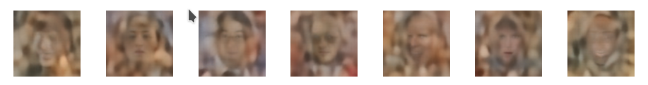
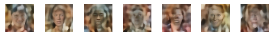
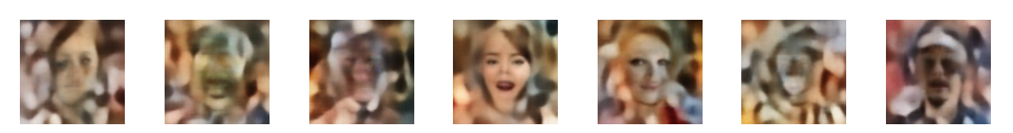
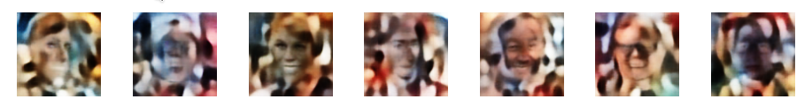
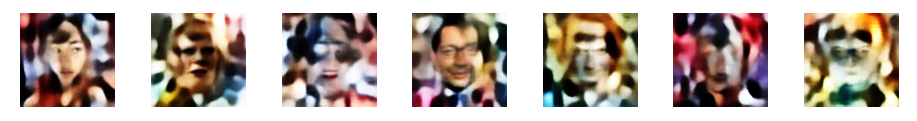
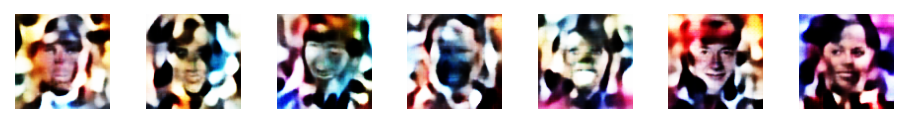
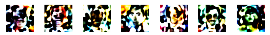
We want to create artificial images of naturally appearing human faces from randomly chosen points in the latent space of a VAE, which has been trained with images of real human faces.
Actually, we will train our VAE with images provided by the so called “Celeb A” dataset. This dataset contains around 200,000 images showing the heads of so called celebrities. Due to the number and size of its images this dataset forces me (due to my very limited hardware) to use a Keras Image Data Generator. A generator is a tool to transfer huge amounts of data in a continuous process and in form of small batches to the GPU during neural network training. The batches must be small enough such that the respective image data fit into the VRAM of the GPU. Our VAE classes have been designed to support a generator.
In this post I first explain why Celeb A poses a thorough test for a VAE. Afterwards I shall bring the Celeb A data into a form suitable for older graphics cards with small VRAM.
Why do the Celeb A images pose a good test case for a VAE?
To answer the question we first have to ask ourselves why we need VAEs at all. Why do certain ML tasks require more than just a simple plain Autoencoder [AE]?
The answer to the latter question lies in the data distribution an AE creates in its latent space. An AE, which is trained for the precise reconstruction of presented images will use a sufficiently broad area/volume of the latent space to place different points corresponding to different imageswith a sufficiently large distance between them. The position in an AE’s latent space (together with the Encode’s and Decoder’s weights) encodes specific features of an image. A standard AE is not forced to generalize sufficiently during training for reconstruction tasks. On the contrary: A good reconstruction AE shall learn to encode as many details of input images as possible whilst filling the latent space.
However: The neural networks of a (V)AE correspond to a (non-linear) mapping functions between multi-dimensional vector spaces, namely
- between the feature space of the input data objects and the AE’s latent space
- and also between the latent space and the reconstruction space (normally with the same dimension as the original feature space for the input data).
This poses some risks whenever some tasks require to use arbitrary points in the latent space. Let us, e.g., look at the case of images of certain real objects in font of varying backgrounds:
During the AE’s training we map points of a high-dimensional feature-space for the pixel values of (colored) images to points in the multi-dimensional latent space. The target region in the latent space stemming from regions in the original feature-space which correspond to “reasonable” images displaying real objects may cover only a relatively thin, wiggled manifold within in the latent space (z-space). For points outside the curved boundaries of such regions in z-space the Decoder may not give you clear realistic and interpretable images.
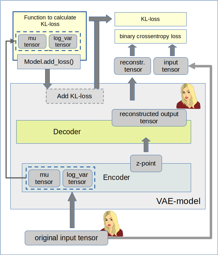
The most important objectives of invoking the KL-loss as an additional optimization element by a VAE are
- to confine the data point distribution, which the VAE’s Encoder part produces in the multidimensional latent space, around the origin O of the z-space – as far as possible symmetrically and within a very limited distance from O,
- to normalize the data distribution around any z-point calculated during training. Whenever a real training object marks the center of a limited area in latent space then reconstructed data objects (e.g. images) within such an area should not be too different from the original training object.
I.e.: We force the VAE to generalize much more than a simple AE.
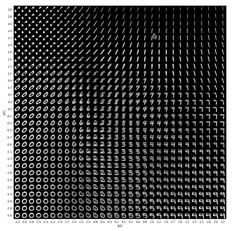
Both objectives are achieved via specific parameterized parts of the KL-loss. We optimize the KL-loss parameters – and thus the data distribution in the latent space – during training. After the training phase we want the VAE’s Decoder to behave well and smoothly for neighboring points in extended areas of the latent space:
The content of reconstructed objects (e.g. images) resulting from neighboring points within limited z-space areas (up to a certain distance from the origin) should vary only smoothly.
The KL loss provides the necessary smear-out effect for the data distribution in z-space.
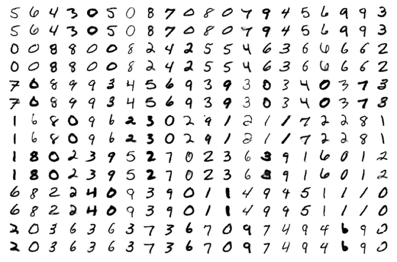
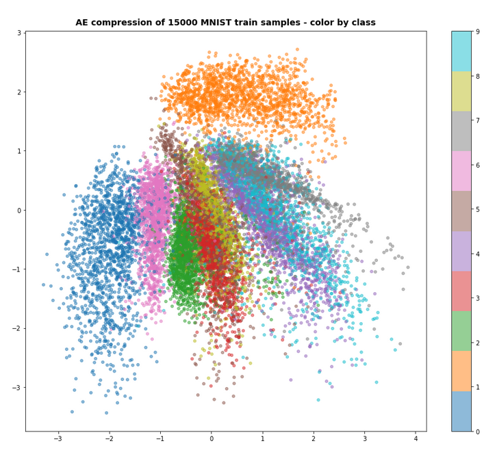
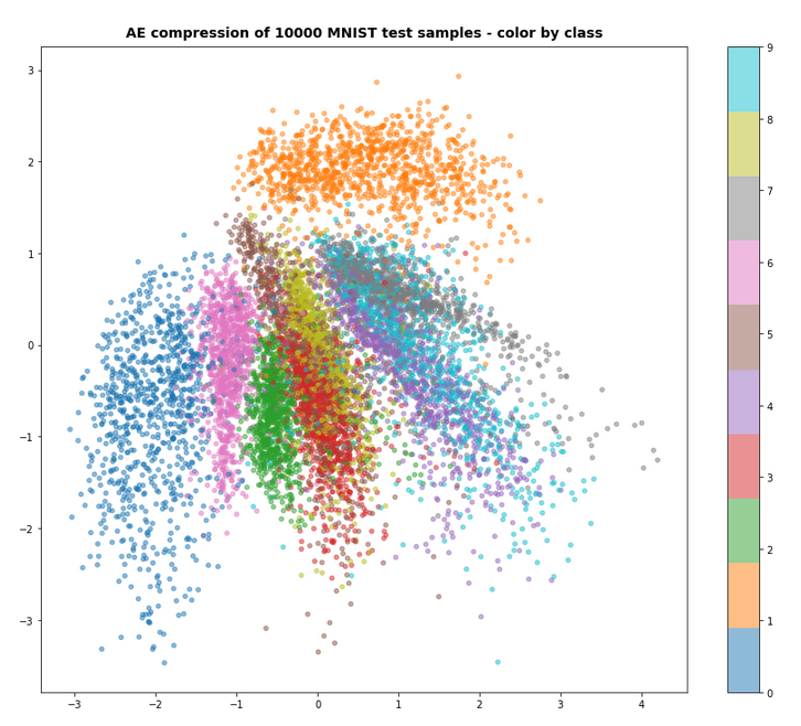
During this series I have only shown you the effects of the KL-loss on MNIST data for a dimension of the latent space z_dim = 2. We saw the general confinement of z-points around the origin and also a confinement of points corresponding to different MNIST-numbers (= specific features of the original images) in limited areas. With some overlaps and transition regions for different numbers.
But note: The low dimension of the latent space in the MNIST case (between 2 and 16) simplifies the confinement task – close to the origin there are not many degrees of freedom and no big volume available for the VAE Encoder. Even a standard AE would be rather limited when trying to vastly distribute z-points resulting from MNIST images of different digits.
However, a more challenging task is posed by the data distribution, which a (V)AE creates e.g. of images showing human heads and faces with characteristic features in front of varying backgrounds. To get a reasonable image reconstruction we must assign a much higher number of dimensions to the latent space than in the MNIST case: z_dim = 256 or z_dim = 512 are reasonable values at the lower end!
Human faces or heads with different hair-dos are much more complex than digit figures. In addition the influence of details in the background of the faces must be handled – and for our objective be damped. As we have to deal with many more dimensions of the z-space than in the MNIST case a simple standard AE will run into trouble:
Without the confinement and local smear-out effect of the KL-loss only tiny and thin areas of the latent space will correspond to reconstructions of human-like “faces”. I have discussed this point in more detail also in the post
Autoencoders, latent space and the curse of high dimensionality – I
As a result a standard AE will NOT reconstruct human faces from randomly picked z-points in the latent space. So, an AE will fail on the challenge posed in the introduction of this post.
Celeb A and the necessity to use a “generator” for the Celeb A dataset on graphics cards with small VRAM
I recommend to get the Celeb A data from some trustworthy Kaggle contributor – and not from the original Chinese site. You may find cropped images e.g. at here. Still check the image container and the images carefully for unwanted add-ons.
The Celeb A dataset contains around 200,000 images of the heads of celebrities with a resolution of 218×178 pixels. Each image shows a celebrity face in front of some partially complex background. The amount of data to be handled during VAE training is relatively big – even if you downscale the images. The whole set will not fit into the limited VRAM of older graphics cards as mine (GTX960 with 4 GB, only). This post will show you how to deal with this problem.
You may wonder why the Celeb A dataset poses a problem as the original data only consume about 1.3 GByte on a hard disk. But do not forget that we need to provide floating point tensors of size (height x width x 3 x 32Bit) instead of compressed integer based jpg-information to the VAE algorithm. You can do the math on your own. In addition: Working with multiple screens and KDE on Linux may already consume more than 1 GB of our limited VRAM.
How can we deal with the Celeb A images on GPUs with limited VRAM ?
We use three tricks to work reasonably fast with the Celeb A data on a Linux systems with limited VRAM, but with around 32 GB or more standard RAM:
- We first crop and downscale the images – in my case to 96×96 pixels.
- We save a binary of a Numpy array of all images on a SSD and read it into the RAM during Jupyter experiments.
- We then apply a so called Keras Image Data Generator to transfer the images to the graphics card when required.
The first point reduces the amount of MBytes per image. For basic experiments we do not need the full resolution.
The second point above is due to performance reasons: (1) Each time we want to work with a Jupyter notebook on the data we want to keep the time to load the data small. (2) We need the array data already in the system’s RAM to transfer them efficiently and in portions to the GPU.
A “generator” is a Keras tool which allows us to deliver input data for the VAE training in form of a continuously replenished dataflow from the CPU environment to the GPU. The amount of data provided with each transfer step to the GPU is reduced to a batch of images. Of course, we have to choose a reasonable size for such a batch. It should be compatible with the training batch size defined in the VAE-model’s fit() function.
A batch alone will fit into the VRAM whereas the whole dataset may not. The control of the data stream costs some overhead time – but this is better than not top be able to work at all. The second point helps to accelerate the transfer of data to the GPU significantly: A generator which sequentially picks data from a hard disk, transfers it to RAM and then to VRAM is too slow to get a convenient performance in the end.
Each time before we start VAE applications on the Jupyter side, we first fill the RAM with all image data in tensor-like form. From a SSD the totally required time should be small. The disadvantage of this approach is the amount of RAM we need. In my case close to 20 GB!
Cropping and resizing Celeb A images
We first crop each of the original images to reduce background information and then resize the result to 96×96 px. D. Foster uses 128×128 px in his book on “Generative Deep Learning”. But for small VRAM 96×96 px is a bit more helpful.
I also wanted the images to have a quadratic shape because then one does not have to adjust the strides of
the VAE’s CNN Encoder and Decoder kernels differently for the two geometrical dimensions. 96 px in each dimension is also a good number as it allows for exactly 4 layers in the VAE’s CNNs. Each of the layers then reduces the resolution of the analyzed patterns by a factor of 2. At the innermost layer of the Encoder we deal with e.g. 256 maps with an extension of 6×6.
Cropping the original images is a bit risky as we may either cut some parts of the displayed heads/faces or the neck region. I decided to cut the upper part of the image. So I lost part of the hair-do in some cases, but this did not affect the ability to create realistic images of new heads or faces in the end. You may with good reason decide differently.
I set the edge points of the cropping region to
top=40, bottom = 0, left=0, right=178 .
This gave me quadratic pictures. But you may choose your own parameters, of course.
A loop to crop and resize the Celeb A images
To prepare the pictures of the Celeb A dataset I used the PIL library.
import os, sys, time
import numpy as np
import scipy
from glob import glob

import PIL as PIL
from PIL import Image
from PIL import ImageFilter

import matplotlib as mpl
from matplotlib import pyplot as plt
from matplotlib.colors import ListedColormap
import matplotlib.patches as mpat
A Juyter cell with a loop to deal with almost all CelebA images would then look like:
Jupyter cell 1
dir_path_orig = 'YOUR_PATH_TO_THE_ORIGINAL_CELEB A_IMAGES'
dir_path_save = 'YOUR_PATH_TO_THE_RESIZED_IMAGES'

num_imgs = 200000 # the number of images we use

print("Started loop for images")
start_time = time.perf_counter()

# cropping corner positions and new img size
left  = 0;   top = 40
right = 178; bottom = 218
width_new  = 96
height_new = 96

# Cropping and resizing
for num in range(1, num_imgs):
    jpg_name ='{:0>6}'.format(num)
    jpg_orig_path = dir_path_orig + jpg_name +".jpg"
    jpg_save_path = dir_path_save + jpg_name +".jpg"
    im = Image.open(jpg_orig_path)
    imc = im.crop((left, top, right, bottom))
    #imc = imc.resize((width_new, height_new), resample=PIL.Image.BICUBIC)
    imc = imc.resize((width_new, height_new), resample=PIL.Image.LANCZOS)
    imc.save(jpg_save_path, quality=95)  # we save with high quality
    im.close()

end_time = time.perf_counter()
cpu_time = end_time - start_time
print()
print("CPU-time: ", cpu_time)
Note that we save the images with high quality. Without the quality parameter PIL’s save function for a jpg target format would reduce the given quality unnecessarily and without having a positive impact on the RAM or VRAM consumption of the tensors we have to use in the end.
The whole process of cropping and resizing takes about 240 secs on my old PC without any parallelized operations on the CPU. The data were read from a standard old hard disk and not a SSD. As we have to make this investment of CPU time only once I did not care about optimization.
Defining paths and parameters to control loading/preparing CelebA images
To prepare and save a huge Numpy array which contains all training images for our VAE we first need to define some parameters. I normally use 170,000 images for training purposes and around 10,000 for tests.
Jupyter cell 2
# Some basic parameters
# ~~~~~~~~~~~~~~~~~~~~~~~~
INPUT_DIM          = (96, 96, 3)
BATCH_SIZE         = 128

# The number of available images
# ~~~~~~~~~~~~~~~~~~~~~~~~~~~~~~~~~
num_imgs = 200000  # Check with notebook CelebA

# The number of images to use during training and for tests
# ~~~~~~~~~~~~~~~~~~~~~~~~~~~~~~~~~~~~~~~~~~~~~~~~~~~~~~~~~~~
NUM_IMAGES_TRAIN  = 170000   # The number of images to use in a Trainings Run
#NUM_IMAGES_TO_USE  = 60000   # The number of images to use in a Trainings Run

NUM_IMAGES_TEST = 10000   # The number of images to use in a training Run

# for historic compatibility reasons of other code-fragments (the reader may not care too much about it)
N_ImagesToUse        = NUM_IMAGES_TRAIN
NUM_IMAGES           = NUM_IMAGES_TRAIN
NUM_IMAGES_TO_TRAIN  = NUM_IMAGES_TRAIN   # The number of images to use in a Trainings Run
NUM_IMAGES_TO_TEST   = NUM_IMAGES_TEST  # The number of images to use in a Test Run

# Define some shapes for Numpy arrays with all images for training
# ~~~~~~~~~~~~~~~~~~~~~~~~~~~~~~~~~~~~~~~~~~~~~~~~~~~~~~~~~~~~~~~~~~~~
shape_ay_imgs = (N_ImagesToUse, ) + INPUT_DIM
print("Assumed shape for Numpy array with train imgs: ", shape_ay_imgs)

shape_ay_imgs_test = (NUM_IMAGES_TO_TEST, ) + INPUT_DIM
print("Assumed shape for Numpy array with test  imgs: ",shape_ay_imgs_test)
We also need to define some parameters to control the following aspects:
- Do we directly load Numpy arrays with train and test data?
- Do we load image data and convert them into Numpy arrays?
- From where do we load image data?
The following Jupyter cells help us:
Jupyter cell 3
# Set parameters where to get the image data from
# ************************************************
# Use the cropped 96x96 HIGH-Quality images
b_load_HQ = True

# Load prepared Numpy-arrays
# ~~~~~~~~~~~~~~~~~~~~~~~~~+
b_load_ay_from_saved = False     # True: Load prepared x_train and x_test Numpy arrays

# Load from SSD
# ~~~~~~~~~~~~~~~~~~~~~~
b_load_from_SSD   = True

# Save newly calculated x_train, x_test-arrays in binary format onto disk
# ~~~~~~~~~~~~~~~~~~~~~~~~~~~~~~~~~~~~~~~~~~~~~~~~~~~~~~~~~~~~~~~~~~~~~~~
b_save_to_disk = False

# Paths
# ******

# Images on SSD
# ~~~~~~~~~~~~~
if b_load_from_SSD:
    if b_load_HQ:
        dir_path_load = 'YOUR_PATH_TO_HQ_DATA_ON_SSD/'    # high quality
    else:
        dir_path_load = 'YOUR_PATH_TO_HQ_DATA_ON_HD/'               #  low quality

# Images on slow HD
# ~~~~~~~~~~~~~~~~~~
if not b_load_from_SSD:
    if b_load_HQ:
        # high quality on slow Raid
        dir_path_load = 'YOUR_PATH_TO_HQ_DATA_ON_HD/'
    else:
        # low quality on slow HD
        dir_path_load = 'YOUR_PATH_TO_HQ_DATA_ON_HD/'


# x_train, x_test arrays on SSD
# ~~~~~~~~~~~~~~~~~~~~~~~~~~~~~
if b_load_from_SSD:
    dir_path_ay = 'YOUR_PATH_TO_Numpy_ARRAY_DATA_ON_SSD/'
    if b_load_HQ:
        path_file_ay_train = dir_path_ay + "celeba_200tsd_norm255_hq-x_train.npy"
        path_file_ay_test  = dir_path_ay + "celeba_200tsd_norm255_hq-x_test.npy"
    else:
        path_file_ay_train = dir_path_ay + "celeba_200tsd_norm255_lq-x_train.npy"
        path_file_ay_test  = dir_path_ay + "celeba_200tsd_norm255_lq-x_est.npy"


# x_train, x_test arrays on slow HD
# ~~~~~~~~~~~~~~~~~~~~~~~~~~~~~~~~~~~
if not b_load_from_SSD:
    dir_path_ay = 'YOUR_PATH_TO_Numpy_ARRAY_DATA_ON_HD/'
    if b_load_HQ:
        path_file_ay_train = dir_path_ay + "celeba_200tsd_norm255_hq-x_train.npy"
        path_file_ay_test  = dir_path_ay + "celeba_200tsd_norm255_hq-x_test.npy"
    else:
        path_file_ay_train = dir_path_ay + "celeba_200tsd_norm255_lq-x_train.npy"
        path_file_ay_test  = dir_path_ay + "celeba_200tsd_norm255_lq-x_est.npy"
You must of course define your own paths and names.
Note that the ending “.npy” defines the standard binary format for Numpy data.
Preparation of Numpy array for CelebA images
In case that I want to prepare the Numpy arrays (and not load already prepared ones from a binary) I make use of the following straightforward function:
Jupyter cell 4
def load_and_scale_celeba_imgs(start_idx, num_imgs, shape_ay, dir_path_load):

    ay_imgs = np.ones(shape_ay, dtype='float32')
    end_idx = start_idx + num_imgs

    # We open the images and transform them into Numpy arrays
    for j in range(start_idx, end_idx):
        idx = j - start_idx
        jpg_name ='{:0>6}'.format(j)
        jpg_orig_path = dir_path_load + jpg_name +".jpg"
        im = Image.open(jpg_orig_path)

        # transfrom data into a Numpy array
        img_array = np.array(im)
        ay_imgs[idx] = img_array
        im.close()

    # scale the images
    ay_imgs = ay_imgs / 255.

    return ay_imgs
We call this function for training images as follows:
Jupyter cell 5
# Load training images from SSD/HD and prepare Numpy float32-arrays
#               - (18.1 GByte of RAM required !! Int-arrays)
#               - takes around 30 to 35 Secs
# ************************************

if not b_load_ay_from_saved:

    # Prepare float32 Numpy array for the training images
    # ~~~~~~~~~~~~~~~~~~~~~~~~~~~~~~~~~~~~~~~~~~~~~~~~~~~~
    start_idx_train = 1
    print("Started loop for training images")
    start_time = time.perf_counter()
    x_train = load_and_scale_celeba_imgs(start_idx = start_idx_train,
                                         num_imgs=NUM_IMAGES_TRAIN,
                                         shape_ay=shape_ay_imgs_train,
                                         dir_path_load=dir_path_load)

    end_time = time.perf_counter()
    cpu_time = end_time - start_time
    print()
    print("CPU-time for array of training images: ", cpu_time)
    print("Shape of x_train: ", x_train.shape)

    # Plot an example image
    plt.imshow(x_train[169999])
And for test images:
Jupyter cell 6
# Load test images from SSD/HD and prepare Numpy float32-arrays
# ~~~~~~~~~~~~~~~~~~~~~~~~~~~~~~~~~~~~~~~~~~~~~~~~~~~~~~~~~~~~~
if not b_load_ay_from_saved:
# Prepare Float32 Numpy array for test images
# ~~~~~~~~~~~~~~~~~~~~~~~~~~~~~~~~~~~~~~~~~~~~
start_idx_test = NUM_IMAGES_TRAIN + 1
print("Started loop for test images")
start_time = time.perf_counter()
x_test = load_and_scale_celeba_imgs(start_idx = start_idx_test,
num_imgs=NUM_IMAGES_TEST,
shape_ay=shape_ay_imgs_test,
dir_path_load=dir_path_load)
end_time = time.perf_counter()
cpu_time = end_time - start_time
print()
print("CPU-time for array of test images: ", cpu_time)
print("Shape of x_test: ", x_test.shape)
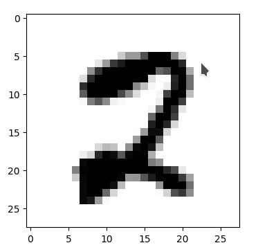
#Plot an example img
plt.imshow(x_test[27])
This takes about 35 secs in my case for the training images (170,000) and about 2 secs for the test images. Other people in the field use much lower numbers for the amount of training images.
If you want to save the Numpy arrays to disk:
Jupyter cell 7
# Save the newly calculatd NUMPY arrays in binary format to disk
# ****************************************************************
if not b_load_ay_from_saved and b_save_to_disk:
    print("Start saving arrays to disk ...")
    np.save(path_file_ay_train, x_train)
    print("Finished saving the train img array")
    np.save(path_file_ay_test, x_test)
    print("Finished saving the test img array")
If we wanted to load the Numpy arrays with training and test data from disk we would use the following code:
Jupyter cell 8
# Load the Numpy arrays with scaled Celeb A directly from disk
# ~~~~~~~~~~~~~~~~~~~~~~~~~~~~~~~~~~~~~~~~~~~~~~~~~~~~~~~~~~~~~~
print("Started loop for test images")
start_time = time.perf_counter()

x_train = np.load(path_file_ay_train)
x_test  = np.load(path_file_ay_test)

end_time = time.perf_counter()
cpu_time = end_time - start_time
print()
print("CPU-time for loading Numpy arrays of CelebA imgs: ", cpu_time)
print("Shape of x_train: ", x_train.shape)
print("Shape of x_test:  ", x_test.shape)
This takes about 2 secs on my system, which has enough and fast RAM. So loading a prepared Numpy array for the CelebA data is no problem.
Defining the generator
Easy introductions to Keras’ ImageDataGenerators, their purpose and usage are given here and here.
ImageDataGenerators can not only be used to create a flow of limited batches of images to the GPU, but also for parallel operations on the images coming from some source. The latter ability is e.g. very welcome when we want to create additional augmented images data. The sources of images can be some directory of image files or a Python data structure. Depending on the source different ways of defining a generator object have to be chosen. The ImageDataGenerator-class and its methods can also be customized in very many details.
If we worked on a directory we might have to define our generator similar to the following code fragment
    data_gen = ImageDataGenerator(rescale=1./255) # if the image data are not scaled already for float arrays
    # class_mode = 'input' is used for Autoencoders
    # see https://vijayabhaskar96.medium.com/tutorial-image-classification-with-keras-flow-from-directory-and-generators-95f75ebe5720
    data_flow = data_gen.flow_from_directory(directory = YOUR_PATH_TO_ORIGINAL IMAGE DATA
                                             #, target_size = INPUT_DIM[:2]
                                             , batch_size = BATCH_SIZE
                                             , shuffle = True
                                             , class_mode = 'input'
                                             , subset = "training"
                                             )
This would allow us to read in data from a prepared sub-directory “YOUR_PATH_TO_ORIGINAL IMAGE DATA/train/” of the file-system and scale the pixel data at the same time to the interval [0.0, 1.0]. However, this approach is too slow for big amounts of data.
As we already have scaled image data available in RAM based Numpy arrays both the parameterization and the usage of the Generator during training is very simple. And the performance with RAM based data is much, much better!
So, how to our Jupyter cells for defining the generator look like?
Jupyter cell 9
# Generator based on Numpy array for images in RAM
# ~~~~~~~~~~~~~~~~~~~~~~~~~~~~~~
b_use_generator_ay = True
BATCH_SIZE    = 128
SOLUTION_TYPE = 3

if b_use_generator_ay:
    # solution_type == 0 works with extra layers and add_loss to control the KL loss
    # it requires the definition of "labels" - which are the original images
    if SOLUTION_TYPE == 0:
        data_gen = ImageDataGenerator()
        data_flow = data_gen.flow(
                           x_train
                         , x_train
                         #, target_size = INPUT_DIM[:2]
                         , batch_size = BATCH_SIZE
                         , shuffle = True
                         #, class_mode = 'input'   # Not working with this type of generator
                         #, subset = "training"    # Not required
                         )
    if ....
    if ....

    if SOLUTION_TYPE == 3:
        data_gen = ImageDataGenerator()
        data_flow = data_gen.flow(
                           x_train
                         #, x_train
                         #, target_size = INPUT_DIM[:2]
                         , batch_size = BATCH_SIZE
                         , shuffle = True
                         #, class_mode = 'input'   # Not working with this type of generator
                         #, subset = "training"    # Not required
                         )
Besides the method to use extra layers with layer.add_loss() (SOLUION_TYPE == 0) I have discussed other methods for the handling of the KL-loss in previous posts. I leave it to the reader to fill in the correct statements for these cases. In our present study we want to use a GradientTape()-based method, i.e. SOLUTION_TYPE = 3. In this case we do NOT need to pass a label-array to the Generator. Our gradient_step() function is intelligent enough to handle the loss calculation on its own! (See the previous posts).
So it is just
        data_gen = ImageDataGenerator()
        data_flow = data_gen.flow(
                           x_train
                         , batch_size = BATCH_SIZE
                         , shuffle = True
                         )
which does a perfect job for us.
In the end we will only need the following call when we want to train our VAE-model
MyVae.train_myVAE(
             data_flow
            , b_use_generator = True
            , epochs = n_epochs
            , initial_epoch = INITIAL_EPOCH
            )
to train our VAE-model. This class function in turn will internally call something like
    self.model.fit(
        data_flow   # coming as a batched dataflow from the outside generator
        , shuffle = True
        , epochs = epochs
        , batch_size = batch_size # best identical to the batch_size of data_flow
        , initial_epoch = initial_epoch
    )
But the setup of a reasonable VAE-model for CelebA images and its training will be the topic of the next post.
Conclusion
What have we achieved? Nothing yet regarding VAE results. However, we have prepared almost 200,000 CelebA images such that we can easily load them from disk into a Numpy float32 array with 2 seconds. Around 20 GB of conventional PC RAM is required. But this array can now easily be used as a source of VAE training.
Furthermore I have shown that the setup of a Keras “ImageDataGenerator” to provide the image data as a flow of batches fitting into the GPU’s VRAM is a piece of cake – at least for our VAE objectives. We are well prepared now to apply a VAE-algorithm to the CelebA data – even if we only have an old graphics card available with limited VRAM.
In the next post of this series
I show you the code for VAE-training with CelebA data. Afterward we will pick random points in the latent space and create artificial images of human faces.
Variational Autoencoder with Tensorflow – X – VAE application to CelebA images
People interested in data augmentation should have a closer look at the parameterization options of the ImageDataGenerator-class.
Links
Celeb A
https://datagen.tech/guides/image-datasets/celeba/
Data generators
https://stanford.edu/~shervine/blog/keras-how-to-generate-data-on-the-fly
towardsdatascience.com/ keras-data-generators-and-how-to-use-them-b69129ed779c
And last not least my standard statement as long as the war in Ukraine is going on:
Ceterum censeo: The worst fascist, war criminal and killer living today is the Putler. He must be isolated at all levels, be denazified and sooner than later be imprisoned. Long live a free and democratic Ukraine!