Einer unserer Kunden will mit LibreOffice Calc/Base direkt auf der Maria/MySQL-Datenbank eines von uns betreuten Linux-LAMP-Servers (unter Opensuse 12.3) arbeiten. Gefordert ist der Datenbankzugang von Opensuse-Linux-Clients wie auch “Windows 7”-Clients aus. Der Server wird bei einem Provider gehostet und für Simulationsberechnungen genutzt. Der Zugang soll aus dem Ausland über das Internet erfolgen. Auf dem Server ist eine Firewall aktiviert. Der Kunde soll die Verbindung selbständig initiieren können.
Ein solches Vorhaben stellt einen vor ein paar sicherheitstechnische Herausforderungen:
- Da die mit der Datenbank auszutauschenden Daten geschäftsrelevant sind, muss die Verbindung verschlüsselt werden. Hierfür bietet sich SSH an.
- Da der Server im Internet gehostet ist, wollen wir keinen weiteren Port außer einem für die Server-Administration sowieso erforderlich SSH-Port und einem für Webanwendungen geöffneten HTTPS-Port von außen zugänglich machen.
- Der Zugang soll nur ganz bestimmten autorisierten Clients zugestanden werden.
- Kundenmitarbeiter sollen nur den Port 3306 der MariaDB-Datenbank, aber keine anderen Ports ansprechen können.
- Die unpriviligierten User-Accounts, unter denen Mitarbeiter des Kunden Verbindung zum Server aufnehmen, dürfen keinen Shell-Zugang erhalten und keine Kommandos absetzen können. Im besonderen dürfen sie keine “Reverse SSH Tunnel” vom Server aus aufzubauen.
- Für Administratoren des Servers erlaubtes SSH Port Forwarding (und damit auch der Aufbau von Reverse SSH Tunnel) darf nicht durch andere Remote Hosts genutzt werden können – auch nicht, wenn die Firewall des Servers mal unten sein sollte.
- Kundenmitarbeiter sollen keine Files per FTP, SCP etc. auf den Server laden können. X11 Forwarding soll unter SSH nicht erlaubt sein.
- Für Tests sollen die Kundenmitarbeiter ihre eigenen Maschinen aber durchaus für einen externen Zugang vom Server aus öffnen dürfen. Sie selbst sollen also für Ihre Hosts einen Reverse SSH Tunnel aufbauen und z.B. ihren eigenen SSH-Port auf den Server exportieren dürfen.
Zur Erfüllung der Anforderungen bieten sich folgende Ansätze an:
- eine SSH-Verbindung – “SSH-Tunnel” – durch die Firewall des Servers,
- “Lokales Port Forwarding” von bestimmten Client-Systemen des Kunden zum Server,
- die Etablierung drastischer Einschränkungen für die SSH-Verbindung,
- die Verhinderung eines Shell Zugangs für die SSH-Nutzer.
Bei all dem gehen wir von “SSH 2”-fähigen Clients und Servern aus.
Angemerkt sei, dass man die ganze Aufgabe ansatzweise auch mit sog. “SSH Reverse Tunnels” (Reverse Port Forwarding) lösen könnte. Dabei würden Ports aktiv vom Server zu definierten Clients exportiert. Ein solches Vorgehen hätte den Vorteil, dass der Zugang vom Server aus eröffnet würde. Dadurch hätte man Kontrolle darüber, wann und zu welchem System die Verbindung aufgebaut wird. Dem entgegen stehen aber etliche praktische, organisatorische Punkte sowie Sicherheitsaspekte. Ein solches Vorgehen ist zudem kaum vereinbar mit der Forderung, dass die Verbindung jederzeit vom Client aus aufgebaut und wieder geschlossen werden können soll. Ich diskutiere deshalb in diesem Blog-Beitrag ein Vorgehen, bei dem ein SSH-basiertes “Local Port Forwarding” von den Kundensystemen aus verwendet wird.
Wir befassen uns dabei vor allem mit Restriktionen der erforderlichen SSH-Konfiguration auf dem Server. Für die geforderten Windows Client zeigen wir in einem
kommenden Teil II ergänzend die PuTTY-Konfiguration für die SSH-Tunnel-Verbindung.
Vorspann: Warum Shell-Zugang und SSH Reverse Tunneling durch die Anwender verhindern ?
Wie viele andere sicherheitsrelevante Tools hat SSH zwei Seiten:
Einerseits eröffnet SSH verschlüsselte Verbindungen zu einem Server oder Host. Dies ist ein Beitrag zur Sicherheit. Andererseits kann SSH aber von kundigen Anwendern auf einem Server oder Host auch dazu genutzt werden, Tunnel durch Firewalls zu graben und die Sicherheit grundlegend zu unterminieren. SSH-Verbindungen, die von einem zu sichernden Server nach außen durch eine Firewall aufgebaut werden können, sind dabei das größte Problem.
Solche Verbindungen können für permanente SSH-Reverse-Tunnel zu externen Maschinen genutzt werden. Dabei wird ein Port des Servers auf die externe Maschine exportiert. Wird ein einmal vom Server aus aufgebauter Reverse SSH-Tunnel später von außen von einem an den Tunnel angebundenen Host genutzt, so wird die Server-Firewall nichts dagegen haben, weil die Nutzung als legitime Antwort auf eine von innen nach außen aufgebaute SSH-Verbindung angesehen wird. Im Zuge eines solchen Tunnels wird gerade die Verschlüsselung zum Problem – es ist im Schadensfall nicht ganz so einfach nachzuweisen, welche Files und Daten durch einen solchen Tunnel vom Server zu Unbefugten transferiert werden.
Die Kombination von Shell-Zugang und SSH-Fähigkeit für Nutzer eines (gehosteten) Servers steht daher im direkten Gegensatz zum Schutz des Servers vor eingehenden Verbindungen von außen. Hierbei nutzt es übrigens auch nichts, den SSH-Port für eine Verbindung vom Server nach außen durch eine Firewall zu sperren – ein SSH-berechtigter Benutzer kann z.B. auch einen nach außen offenen HTTPS-Port (443) für SSH-Operationen nutzen. Meine Devise ist daher:
SSH ist für die meisten regulären Benutzer zu schützender Systeme grundsätzlich nicht zuzulassen – im besonderen nicht mit der Option, Ports “forwarden” zu dürfen.
Wir befinden uns deshalb in einem Dilemma, denn unseren externen Kunden-Mitarbeitern müssen wir einen SSH-Zugang mit Port-Forwarding zugestehen. Wir lösen das Dilemma dadurch, dass diese User auf dem Server weder mit Hilfe von SSH noch sonstwie Kommandos absetzen, noch dass sie persönliche “ssh_config” anlegen oder modifizieren können:
Externen Anwendern, denen ein SSH-Zugang zu einem bestimmten Service (Port) eines zu schützenden, gehosteten Servers gewährt wird, darf in keinem Fall ein (SSH-) Zugang zu einer Shell eingeräumt werden. Externe Anwender mit SSH-Tunnel-Zugang sind ja de facto User auf dem Server, denen die SSH-Verbindung explizit – und wie wir sehen werden, mit “Port Forwarding” – zugestanden wird. Ein solcher SSH-Benutzer mit Shell-Zugang würde eine echte Gefahr für die Sicherheit darstellen. Sie sollen mit SSH deshalb ausschließlich einen Tunnel von ihren Hosts zum Server aufbauen können (Local Port Forwarding). Sonst nichts ….
Einschränkung des Zugangs auf bestimmte Clients
Die Begrenzung des des SSH-Zugangs auf bestimmte Clients haben wir durch folgende Maßnahmen erreicht:
- "Umkonfiguration" des SSH-Zugangs auf eine gegenüber dem Standard modifizierte Port-Nummer. Den Clients muss diese Nummer bekannt sein. [Kein echter Schutz, aber eine erste Hürde für Angreifer und Skript-Kiddies … siehe die Anmerkung weiter unten]
- Einschränkung des Serverzugangs auf genau diesen einen Port (neben https) über eine Firewall.
- Einschränkungen des SSH-Zugangs auf bestimmte IP-Client-Adressen über eine
entsprechend konfigurierte Firewall. - Vollständiger Ersatz des passwort-basierten Zugangs durch eine Authentisierung der Clients gegenüber dem Server, die auf asymmetrischen SSH-RSA-Schlüsseln beruht.
Auf die genaue Firewall-Konfigurationen gehe ich hier nicht ein. Die eingesetzte Firewall schottet sämtliche anderen Ports komplett ab. Angemerkt sei auch, dass wir außer HTTPS-Verbindungen, DNS- und NTP-Verbindungen zu ganz bestimmten Hosts im Internet keine vom Server initiierte Verbindungen nach außen zulassen.
Wie man den ersten und letzten Punkt der obigen Liste (Portmodifikation, schlüsselbasierte Authentifizierung) realisiert , kann man u.a. in entsprechenden Blog-Artikeln zur Konfiguration eines gehosteten (virtuellen) Strato-V-Servers nachlesen:
Strato-V-Server mit Opensuse 12.3 – II – Installation / SSH-Port ändern
Strato-V-Server mit Opensuse 12.3 – III – Stop SSH Root Login
Strato-V-Server mit Opensuse 12.3 – IV – SSH Key Authentication
Siehe aber auch die Links zur schlüsselbasierten Authentifizierung am Ende des Artikels. Der Vorteil von schlüsselbasierten Zugangsverfahren ist die Kombination aus Besitz eines Schlüssels mit einer zusätzlichen Passphrase auf den Client-Systemen. Systeme und User, die über das eine oder andere nicht verfügen, erlangen keinen Zugang zum Server – soweit das asymmetrische Schlüselverfahren selbst keine Backdoors beinhaltet.
Eine Warnung erscheint mir dennoch angebracht:
Eine schlüsselbasierte Zugangsbeschränkung ist im Sinne eines berechtigten Datenzugangs nur genau soweit sicher, als sie den Benutzern, denen die Private Keys zugeordnet werden, trauen können. Verbreiten diese User Ihre Keys, so ist gegen den Datenbank-Zugang anderer externer User kein Kraut gewachsen. Eine Sicherheitsbelehrung mit Androhung entsprechender Sanktionen ist sicher sinnvoll. Für technisch komplexere Lösungen, bei denen die User des Tunnels selbst keinen direkten lesenden Zugang auf zugeordnete “Private Keys” mehr erhalten sollen, siehe den entsprechenden Link im letzten Abschnitt dieses Artikels.
Diese potentielle Gefahr der Schlüsselweitergabe macht es umso mehr erforderlich, weitere Barrieren hochzufahren. Das betrifft zum einen die sowieso erforderliche Verhinderung des Shell-Zugangs der externen SSH-Tunnel-User – aber auch drastische Beschränkung der Userberechtigungen auf der Datenbank selbst. Sich die Rechte auf der Datenbank genau zu überlegen und auf ein Minimum zu beschränken, gehört zum ganzen Setup unbedingt dazu! Auch wenn wir in diesem Artikel nicht darauf eingehen..
Eine Anmerkung noch zur vorgenommenen Verlagerung des SSH-Ports :
Unter bestimmten Bedingungen – z.B. bei aktiven Usern, die Shell-Zugang auf dem LAMP-Server haben – kann es problematisch werden, SSH auf einen unpriviligierten Port zu verschieben. Siehe hierzu den Artikel und die interessante Diskussion unter
why-putting-ssh-on-another-port-than-22-is-bad-idea
Aber:
Wenn es auf dem zu schützenden LAMP-Server keinen normalen User neben dem Admin gibt, der einen unpriviligierten Port nach außen öffnen kann, sehe ich die im angegebenen Artikel diskutierten Gefahren nicht. Die Gefahr einer Umlenkung eines bereits belegten Ports von außen ist unter den in diesem Artikel dargestellten Bedingungen auch nicht gegeben. Somit dient die Port-Änderung einer Abschwächung des ansonsten stattfindenden
externen Dauerbeschusses auf Port 22 oder andere priviligierte Ports durch Verschleierung (“Obfuscating”). Man muss sich allerdings darüber im Klaren sein, dass sukzessive Stealth Portscans (ggf. von verschiedenen Systemen) aus, früher oder später zur Entdeckung des offenen Ports führen werden und damit auch zu Versuchen eines SSH-Zugangs über diesen Port. Dann müssen andere Sicherheitsmaßnahmen greifen – wie eben z.B. die Authentifizierung per Keys und andere Vorkehrungen. “Obfuscating” allein bietet keinen Schutz, sondern stellt maximal eine erste kleine Hürde in einer Kette von Schutzmaßnahmen dar.
Globale Optionen in der Konfigurationsdatei /etc/ssh/sshd_config des Servers
Der Server heiße “kundenserver.de“. Wir setzen nachfolgend voraus, dass der SSH-Zugang auf SSH-Schlüsselpaaren beruht und dem Server alle Public SSH-Keys der zugelassenen Remote-User bekannt sind (Dateien “~/.ssh/authorized_keys”) . Wir haben uns – schon aus Logging-Gründen – dazu entschlossen, den SSH-Zugang für die Kundenmitarbeiter auf mehrere (eingeschränkte) Accounts auf dem Server zu verteilen. Eine Lösung, bei der sich mehrere User des Kunden über genau einen User-Account des Servers einloggen, haben wir verworfen. Auch die Datenbank-User wurden getrennt. Es gibt Vor- und Nachteile beider Lösungen. Beim hier gewählten Verfahren sind u.a. mehr Accounts und ggf. auch Schlüssel zu verwalten. Da es nur um 3 User (“kundea”, “kundeb”, “kundec”) geht, ist der Aufwand aber erträglich.
Wir nutzen nun globale Optionen in der Datei “/etc/ssh/sshd_config” auf dem Server, um einen root-Zugang über SSH zu verhindern und andererseits den SSH-Zugang von außen auf die ausgewählten Kundenmitarbeiter zu beschränken. Ferner wird eine Nutzung von X11 unterbunden. Der offene SSH-Port habe als Beispiel die Nummer "6XXXX". Es ergeben sich dann folgende Einträge in der sshd_config:
“Auszug /etc/ssh/sshd_config“:
Port 6xxxx
PermitRootLogin no
AllowUsers kundea kundeb kundec
RSAAuthentication yes
PubkeyAuthentication yes
AuthorizedKeysFile .ssh/authorized_keys
PasswordAuthentication no
ChallengeResponseAuthentication no
UsePAM no
X11Forwarding no
GatewayPorts no
UsePrivilegeSeparation sandbox
PermitTunnel no
AllowAgentForwarding no
AllowTcpForwarding no
#Subsystem sftp /usr/lib/ssh/sftp-server
Kundige Leser werden sich an dieser Stelle über die Option “AllowTcpForwarding no” wundern. Wir heben diese globale Beschränkung weiter unten user-bezogen wieder auf.
Man beachte auch die Auskommentierung des letzten Eintrags. Es werden keine SSH-Subsysteme wie SFTP zugelassen.
Wir erweitern weiter unten unsere SSH-Einschränkungen noch und gehen dabei auch auf die Einstellung “GatewayPorts no” und “AllowAgentForwarding no” ein.
Testen des SSH-Tunnels vom Linux-Client aus
Nehmen wir an, einer der User unseres Kunden, der Zugang zum (Datenbank-) Server erhalten soll, habe auf unserem Server “kundenserver.de” den Account "kundea". Auf seinem eigenen Linux-Host “kundensystema” habe der Kunde dagegen einen Account “kunda”. Der Host “kundensystema” fungiert als SSH-Client bzgl. des SSH-Servers “kundenserver.de”. Der für unseren Server benutzte “Private SSH RSA Keys” des Users sei auf “kundensystema” in der Datei
~/.ssh/id_a_kundenserver
hinterlegt. Dort gebe es aber noch andere Private
Key Files für andere Server.
Es gelte ferner die Einschränkung, dass der lokale Port "3306" des Linux-Clients “kundensystema” schon durch eine lokale MySQL-Datenbank belegt sei. Der Port "3307" sei dagegen frei. Welches Kommando ist dann auf dem Linux-System “kundensystema” von “kunda” erforderlich, um per SSH-Tunnel auf die Datenbank zu kommen?
Auf der Kommandozeile einer Linux Bash Shell kann man zum Aufbau des benötigten Tunnels Folgendes eingeben:
kunda@kundensystema :~> ssh -fN -L3307:127.0.0.1:3306 \
> kundea@kundenserver.de -p 6xxxx -i ~/.ssh/id_a_kundenserver
(Der Backslash steht für den Zeilenumbruch auf der Kommandozeile !)
“kunda” sollte nun nach der Passphrase des Private Keys gefragt werden. Nach korrekter Eingabe steht der Tunnel durch die Firewall zum Port 3306 des Servers:
Der lokale Client-Port 3307 wird auf dem Server “kundenserver” über den auf Port 6xxxx eröffneten SSH-Tunnel auf den dortigen Port 3306 umgelenkt. Letzteres geschieht quasi durch die aktive Firewall des Servers hindurch. Benötigt wird von außen nur der Zugang zum Port “6xxxx” der SSH-Verbindung.
Zu den Optionen
"-f" ( SSH Prozess wird in den Hintergrund verschoben)
und
"-N" ( “do not execute a remote command” – nur Tunneling !)
ps -aux | grep ssh -fNund nachfolgendem Identifizieren der PID des ssh-Prozess plus
kill -15 PID
Für andere Verfahren zur (skriptbasierten) Beendigung siehe die Links unten.
Testen des Tunnels zur Datenbank mittels “mysql”
Wir wollen nun testen, ob wir vom Host des Kunden aus wirklich über den zuvor geöffneten “Tunnel” zur Datenbank des Servers kommen. Hierzu nutzen wir das Kommandozeilentool "mysql". Der Datenbankaccount für diesen User auf dem Server “kundenserver.de” heiße "sqlkundea".
Unter Linux müssen wir bzgl. des Testens der Remote-Verbindung übers Internet eine kleine Falle umgehen. Es gibt nämlich bzgl. des Zugangs zu einer MySQL-Datenbank einen Unterschied zwischen “localhost” und “127.0.0.1”:
Tools wie mysql versuchen unter Linux bei Angabe von “localhost” eine Verbindung über einen (schnelleren) lokalen UNIX-Domain-Socket statt einer Netzwerk-TCP/IP-Verbindung zum Datenbank-Daemon. [Unter Windows wird dagegen immer eine TCP/IP-Verbindung geöffnet.]
Im hier besprochenen Port-Umlenkungsfall ist eine TCP/IP-Verbindung zur Bank des Servers auch unter Linux zu konfigurieren. Bei Angabe der IP-Adresse 127.0.0.1 wird eine solche geöffnet. Siehe auch:
http://stackoverflow.com/questions/3715925/localhost-vs-127-0-0-1
http://stackoverflow.com/questions/9714899/php-mysql-difference-between-127-0-0-1-and-localhost
http://stackoverflow.com/questions/16134314/mysql-connect-difference-between-localhost-and-127-0-0-1
Beim Testen auf der Kommandozeile der “bash” empfiehlt es sich also,
kunda@
kundensystema :~>mysql -h 127.0.0.1 -u sqlkundea -p
anstatt “… -h localhost…” anzugeben. Steht der Tunnel und haben wir alles richtig gemacht, so gelangen wir (genauer “kunda” auf “kundensystema”) nach Eingabe des Datenbank-Zugangspassworts auf den MariaDB/MySQL-Service “auf kundenserver.de” :
kunda@kundensystema:~> mysql -P 3307 -h 127.0.0.1 -u sqlkundea -p
Enter password:
Welcome to the MariaDB monitor. Commands end with ; or \g.
Your MariaDB connection id is 7308
Server version: 5.5.33-MariaDB openSUSE package
Copyright (c) 2000, 2013, Oracle, Monty Program Ab and others.
Type ‘help;’ or ‘\h’ for help. Type ‘\c’ to clear the current input statement.
MariaDB [(none)]>
Dass man wirklich auf dem Server-RDBMS und nicht einem lokalen MySQL-RDBMS gelandet ist, ergibt sich entweder bereits aus dem server-spezifischen Passwort oder einem anschließenden “connect” zu einer speziellen, nur auf dem Server existierenden Bank.
Weitere Restriktionen auf dem Server – Verhindern des Absetzens von Kommandos
Bislang haben wir zusätzlich zum schlüsselbasierten Zugang lediglich die Firewall des Servers per SSH-durchtunnelt, um an den dortigen 3306-Port zu gelangen. Der User “kundea” kann sich mit den obigen Konfigurationseinstellungen aber noch ganz normal in eine SSH-Shell einloggen und Kommandos absetzen.
kunda@kundensystema:~>ssh kundea@kundenserver.de -p 6xxxx \
> -i ~/.ssh/id_a_kundenserver
Enter passphrase for key ‘/home/kundea/.ssh/id_a_kundenserver’:
Last login: Mon Nov 11 09:18:42 2013 from kundensystem.de
Have a lot of fun…
kundea@kundenserver:~>
Das und weitere Dinge wollen wir nun unterbinden. Das kann man in einem ersten Schritt z.T. durch globale Vorgaben in der “/etc/ssh/sshd_config” erreichen. Wir zeigen zur Abwechslung aber mal ein userspezifisches Vorgehen. Es gibt zwei Methoden, userspezifische Restriktionen des sshd-Daemons auf dem Server wirksam zu machen:
- Zentrale Einstellungen in der Konfigurationsdatei “/etc/ssh/sshd-config”.
- “Public Key”-spezifische Restriktionen in den Files “~/.ssh/authorized_keys” derjenigen Accounts über die der Zugang (hier zum Datenbank-Port) erfolgen soll.
Ich gehe in diesem Beitrag genauer nur auf die erste Variante ein. Man kann die kommenden Restriktionen aber auch den spezifischen Schlüsseln voranstellen, die man in der Datei
~/.ssh/authorized_keys
des Users bzw. derjenigen User auf dem Server, über dessen Account bzw. der Datenbankzugang erfolgen soll, untergebracht hat. Siehe hierzu die Links am Ende des Artikels.
Wir wollen Restriktionen exemplarisch und userspezifisch für den Account “kundea” auf dem Server vornehmen. Für userspezifische Festlegungen in der sshd_config gibt es die Vorgabe “Match User” – hier für unsere Kundenmitarbeiter
Match User kundea kundeb kundec
Siehe hierzu und für andere Varianten von “Match” (z.B. für Usergruppen):
http://linux.die.net/man/5/sshd_config
Ich zitiere zu “Match”:
Introduces a conditional block. If all of the criteria on the Match line are satisfied, the keywords on the following lines override those set in the global section of the config file, until either another Match line or the end of
the file.
Hinter dem “Match”-Statement kann man also Optionen für die SSHD-Parameter angeben, die sich dann userspezifisch auswirken. Unter OpenSSH sind Vorgaben für folgende Parameter möglich:
AllowAgentForwarding, AllowTcpForwarding, Banner, ChrootDirectory, ForceCommand, GatewayPorts, GSSAPIAuthentication, HostbasedAuthentication, KbdInteractiveAuthentication, KerberosAuthentication, KerberosUseKuserok, MaxAuthTries, MaxSessions, PubkeyAuthentication, AuthorizedKeysCommand, AuthorizedKeysCommandRunAs, PasswordAuthentication, PermitEmptyPasswords, PermitOpen, PermitRootLogin, RequiredAuthentications1, RequiredAuthentications2, RhostsRSAAuthentication, RSAAuthentication, X11DisplayOffset, X11Forwarding and X11UseLocalHost.
Außerhalb der userspezifischen Festlegungen für diese Parameter gelten die globalen Einstellungen. Man nimmt userspezifische Einschränkungen am Ende des Konfigurationsfiles vor. Für die von uns geforderten Einschränkungen sind vier Parameter relevant:
Match User kundea kundeb kundec
#X11Forwarding no
#PermitTunnel no
#GatewayPorts no
AllowTcpForwarding yes
PermitOpen 127.0.0.1:3306 localhost:3306
AllowAgentForwarding no
ForceCommand echo ‘This account can only be used for tunneling’
Die auskommentierten Statements geben dabei ergänzend einige Standardeinstellungen von OpenSSH oder von uns explizit vorgenommene globale Einstellungen wieder (s.oben).
Zur Option “AllowTcpForwarding”
Nicht einzuschränken ist an dieser Stelle für die Kunden-Mitarbeiter die Option “AllowTcpForwarding”. Ein Abschalten dieser Option würde jedes Port-Forwarding unterbinden – auch das gewünschte “Local Port Forwarding” unserer Kunden zum Server selbst ! Da wir global kein Port-Forwarding zugelassen haben (auch um Reverse Tunneling zu unterbinden), müssen wir es jetzt user-spezifisch erlauben:
AllowTcpForwarding yes
Zur Option “PermitOpen”
Ich zitiere aus den man-Seiten :
PermitOpen: Specifies the destinations to which TCP port forwarding is permitted. The forwarding specification must be one of the following forms:
PermitOpen host:port
PermitOpen IPv4_addr:port
PermitOpen [IPv6_addr]:port
Multiple forwards may be specified by separating them with whitespace. An argument of “any” can be used to remove all restrictions and permit any forwarding requests. By default all port forwarding requests are permitted.
Dass hier “host” und “port” anzugeben sind, hat damit zu tun, dass das SSH-Port-Forwarding ja nicht zwingend auf unseren Server selbst als Zieladresse beschränkt sein muss, sondern dieser auch als Sprungbrett zu jedem beliebigen anderen Host, zu dem der Server Zugang hat, genutzt werden kann. Wir wollen das Forwarding aber aus Perspektive des angesprochenen SSH-Servers genau auf ihn selbst – also “localhost” – und den Port 3306 begrenzen.
Wir geben in der sshd_config deshalb beide Varianten der localhost-Definition – einmal “wörtlich” und einmal über das Loopback-Interface – an, um unter Windows und Linux den Unterschied, den MySQL-Tools bzgl. des Zugangs evtl. machen, sicher hantieren zu können.
Zur Option “AllowAgentForwarding”
Ich zitiere aus den man-Seiten :
AllowAgentForwarding:
r
Specifies whether ssh-agent(1) forwarding is permitted. The default is “yes”. Note that disabling agent forwarding does not improve security unless users are also denied shell access, as they can always install their own forwarders.
Man kann den Server beim Aufbau einer SSH-Verbindung veranlassen, weitere Keys für Verbindungen zu weiteren Servern aus einem lokal auf dem SSH-Client-System laufenden SSH-Key-Agent auszulesen. Der Server könnte dann als Zwischenstation für Verbindungen zu anderen Servern missbraucht werden. Nicht immer können wir über eine Firewall alle Verbindungen nach außen auf nur wenige Adressen einschränken. Und auch eine Firewall muss ggf. mal abgeschaltet werden. Dann schützt die obige Angabe trotzdem gegen clientbasiertes AgentForwarding.
Zur Option “ForceCommand”
Ich zitiere aus den man-Seiten :
ForceCommand:
Forces the execution of the command specified by ForceCommand, ignoring any command supplied by the client. The command is invoked by using the user’s login shell with the -c option. This applies to shell, command, or subsystem execution. The command originally supplied by the client is available in the SSH_ORIGINAL_COMMAND environment variable.
Damit können wir die Kundenmitarbeiter daran hindern, auf dem Server Kommandos abzusetzen:
ForceCommand echo ‘This account can only be used for tunneling’
Test:
kunda@kundensystema:~> ssh kundea@kundenserver.de -p 6xxxx \
> -i ~/.ssh/id_a_kundenserver
Enter passphrase for key ‘/home/kunde/.ssh/id_rsa’:
This account can only be used for tunneling
Connection to kundenserver.de closed.
Gibt an “-v” als zusätzliche ssh-Option an, so sieht man einen Exit Code 0. Das echo-Kommando wurde fehlerfrei ausgeführt. Mehr ist aber für den Kunden nicht möglich. Trotzdem kann er mit dem Kommando
kunda@kundensystema :~> ssh -fN -L3307:127.0.0.1:3306 \
> kundea@kundenserver.de -p 6xxxx -i ~/.ssh/id_a_kundenserver
nach wie vor den gewünschten Tunnel zur Datenbank aufbauen. (Übrigens: Man kann mit “ForceCommand” in anderen Szenarien viele hübsche Dinge machen, z.B. einen 2 Phasen Login basteln oder den externen User auf genau ein Programm wie etwa “svn” umlenken, etc. . Es lohnt sich wirklich, damit ein wenig zu experimentieren. )
Entzug des Shell-Zugangs
Trotz des Einsatzes von “ForceCommand” sind wir noch nicht ganz zufrieden. Ich sehe es als wichtig an, dem User jedes Recht zu nehmen, sich in eine bedienbare Shell auf dem Server einzuloggen. Ein ggf. später hinzukommender normaler User auf dem Server könnte z.B. versuchen, die Accounts von “kundea”, “kundeb”, “kundec” auf dem Server zu hacken und unter Ihrem Namen einen Reverse SSH Tunnel aufzubauen. Auch das wollen wir verhindern. Dazu muss der Shell-Zugang völlig unterbunden werden. Fehler beim Hochfahren von SSH oder der Konfiguration von SSH sollen nicht ausgenutzt werden können.
Dies erreichen wir als Admin durch :
kundenserver.de:~ # usermod – s /bin/false kundea
und analog für die anderen Accounts. Dies führt zu folgendem Verhalten:
kunda@kundensystema:~> ssh kundea@kundenserver.de -p 6xxxx \
> -i ~/.ssh/id_a_kundenserver
Enter passphrase for key ‘/home/kunde/.ssh/id_rsa’:
Connection to h2215102.stratoserver.net
closed.
kunda@kundensystema:~>
Verwenden wir wieder die Option “-v”, so erkennen wir, dass der Exit Code diesmal “1” ist:
debug1: Exit status 1
Selbst das Absetzen des “echo”-Kommandos schlägt jetzt fehl und die angestrebte SSH-Verbindung wird abgebrochen. Dennoch ist es mit der Option “-fN” immer noch erfolgreich möglich, den Tunnel zur Datenbank herzustellen. Das zugehörige Kommando
kunda@kundensystema :~> ssh -fN -L3307:127.0.0.1:3306 \
> kundea@kundenserver.de -p 6xxxx -i ~/.ssh/id_a_kundenserver
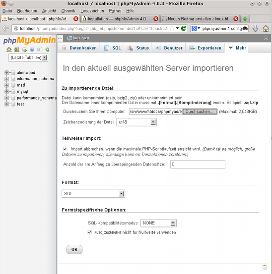
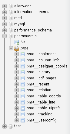
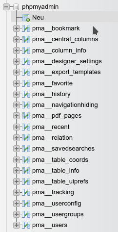
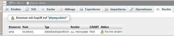
wird anstandslos ausgeführt. Testen kann man den Tunnel natürlich wie oben gezeigt mittels des”mysql”-Tools. Es steht nun weiteren Experimenten mit anderen Datenbank-Tools wie z.B. phpMyAdmin oder BASE aus der LibreOffice-Suite über den Tunnel hinweg nichts mehr im Wege.
Zur Option “GatewayPorts no” auf den SSH-Client-Systemen und dem Server
Zusätzlich checken wir zur Sicherheit, dass sowohl auf den SSH-Client-System “kundensystema”, “kundensystemb”, etc. und auch dem Server die globale Option
GatewayPorts no
wirklich auf “no” gesetzt ist.
Auf den Client-Systemen ist die für die Konfiguration zuständige Datei
/etc/ssh/ssh_config
Dort setzen wir explizit die Option
GatewayPorts no
Zusätzlich setzte der Kunden-Admin dies auch noch in der “sshd_config” der Hostsysteme beim Kunden. Diese Maßnahme dient zum Schutz unserer Kundensysteme, aber auch zum Schutz des Servers:
Die genannte Option steuert, ob andere Hosts mit Verbindung zu den Kundensystemen Zugang zum dort umgeleiteten Port 3307 bekommen sollen oder nicht. Endpunkte von TCP Verbindungen (Sockets !) werden auf Linux-Systemen typischerweise an alle Netzwerkinterfaces gebunden. Die obige Option verhindert das und bindet den (umzulenkenden) Port, auf den das jeweilige Kundensystem hört, ausschließlich an dessen Loopback-Interface. Das Loopback-Interface ist danach nur lokal zugänglich. Damit ist es für externe Hosts und deren User nicht mehr möglich, über Interfaces, die unsere SSH-Client-Systeme mit dem Rest der ihnen zugänglichen Welt verbinden, den Port zu nutzen, der zu unserem Server ge-“forwarded” wird.
Dies verhindert allerdings noch nicht, dass eventuelle andere kundige lokale Benutzer von “kundensystema” diesen umgeleiteten Port nutzen können. Aber ein Unterbinden der Nutzung des Datenbankports durch lokale Nutzer des Servers muss man auf anderem Wege – wie etwa den Einsatz der Keyfiles – erreichen.
Ein Seitenblick auf “Local Port Forwarding” vom Server zu den Client-Systemen
Warum “GatewayPorts no” auf dem Server? Sind mehrere Administratoren auf dem Server aktiv, könnte einer von Ihnen auf den Gedanken kommen, für Tests SSH-Verbindungen vom Server zu definierten Client-Systemen aufzunehmen. Dann würde er ggf. “Local Port Forwarding” zu den Client-Systemen nutzen, die diesen Zugang erlauben. Eine Nutzung umgelenkter Serverports zu irgendwelchen Clients soll natürlich unter keinen Umständen für externe Hosts möglich sein. Und da meinen wir nicht nur die Hosts der Kunden. Wir setzen daher zur Sicherheit auch in der “/etc/ssh/sshd_config” des Servers explizit die Option
GatewayPorts no
Wir hatten ja bereits angemerkt, dass der Server gegen Zugriffe von außen durch eine Firewall geschützt werden soll. Warum also diese explizite Einschränkung? Hierfür gibt es zwei Gründe:
- Auf gehosteten Servern gibt es immer mal wieder Situationen, in denen mit der Firewall kurzfristig gearbeitet und ggf. experimentiert werden muss.
Die vorgenommene Einstellung schützt dann unabhängig von der Firewall. - Auf gehosteten und remote verwalteten Systemen kann es als Notanker erforderlich sein, einen über Verwaltungsoberflächen des Hosters vorgenommenen Reboot ohne unmittelbaren Start von Firewall-Skripten ablaufen zu lassen. Die FW und weitere Server-Dienste werden dann nur zeitverzögert hochgefahren. In der Zwischenzeit steht dann (nur) der modifizierte SSH-Port bereit – aber ohne weitere, zusätzlich Firewall-Einschränkungen. Nach einem Reboot schützt die obige Einstellung auch innerhalb des gewährten Zeitintervalls ohne Firewall.
An solche Szenarien muss man u.U. dann denken, wenn man viel unterwegs ist und man im Notfall auch von einem fremdem System aus unbedingt Zugang zum Server bekommen muss.
Fazit
Wir haben durch die geschilderten Einstellungen alle anfänglich genannten Ziel erreicht. Dass der Kunde über einen Reverse-Tunnel von seinem eigenen Host aus einen eigenen Port auf einen unbesetzten Port des Servers exportieren kann, kann der Leser selbst testen. Hierbei ergibt sich die interessante Frage, ob er dadurch einen bereits besetzten Port übernehmen kann. Dies ist nicht der Fall – zumindest nicht, wenn es nur genau ein Netzwerk-Interface nach außen gibt.
Es ist also möglich, einen kryptierten SSH-Tunnel mit Local Port Forwarding zur MySQL/MariaDB-Datenbank auf einem gehosteten Server (mit Firewall) einzurichten. Gerade die unglaubliche Flexibilität von SSH beim Untergraben von Firewalls macht aber etliche Sicherheitsvorkehrungen im Umfeld der eigentlichen Tunnelverbindung unerlässlich. Aber auch nach dem erforderlichen Unterbinden des Shell-Zugangs auf dem Server können unsere Kunden immer noch den gewünschten reinen Tunnel zur Datenbank aufbauen und nutzen.
Bleibt noch anzumerken, dass man den Kundenmitarbeitern das Arbeiten natürlich noch etwas erleichtern kann, indem man die Port-Forwarding-Optionen in deren ~/.ssh/ssh_config”-Dateien verankert. Zudem wird man – je nach Sicherheitsphilosophie des dortigen Admins ggf. auch “SSH-Agents” einsetzen, damit die Passphrase für das Auth-Key-File nicht so oft eingegeben werden muss. Ferner kann man an Skripts zum vereinfachten Tunnelaufbau denken. Hier ist intensive Kooperation mit dem Kunden-Admin erforderlich.
Im nächsten Beitrag zum getunnelten Datenbankzugang gehe ich auf die erforderliche PuTTY-Konfiguration für potentielle Windows 7 Clients ein.
Links
Key-basierte Authentifizierung
http://linuxwiki.de/OpenSSH
http://sourceforge.net/apps/trac/sourceforge/wiki/SSH%20keys
http://www.lofar.org/wiki/doku.php?id=public:ssh-usage
http://www.ceda.ac.uk/help/users-guide/ssh-keys/
http://docstore.mik.ua/orelly/networking_2ndEd/ssh/ch09_02.htm
http://docstore.mik.ua/orelly/networking_2ndEd/ssh/ch08_02.htm
http://en.wikibooks.org/wiki/OpenSSH/Cookbook/Authentication_Keys
http://www.eng.cam.ac.uk/help/jpmg/ssh/authorized_keys_howto.html
Sicherung gegen Kopieren der Private Keys
Alles andere als einfach. In Unternehmen muss man ggf. zu Lösungen greifen, die zentrale Gateway-Server als Custodians für die SSH-verbindungen einsetzen. Eien entsprechende Lösung ist hier beschrieben:
http://stackoverflow.com/questions/9286622/protecting-ssh-keys
http://martin.kleppmann.com/2013/05/24/improving-security-of-ssh-private-keys.html
SSH-Tunneling und Restriktionen
http://docstore.mik.ua/orelly/networking_2ndEd/ssh/ch09_02.htm#ch09-17854.html
http://www.debianadmin.com/howto-use-ssh-local-and-remote-port-forwarding.html
http://en.wikibooks.org/wiki/OpenSSH/Cookbook/Tunnels
http://bioteam.net/2009/10/ssh-tunnels-for-beginners/
http://bioteam.net/2009/11/ssh-tunnels-part-3-reverse-tunnels/
http://snajsoft.com/2009/02/12/prevent-reverse-ssh/
https://raymii.org/s/tutorials/Autossh_persistent_tunnels.html
http://www.spencerstirling.com/computergeek/sshtunnel.html
http://freddebostrom.wordpress.com/2009/04/10/ssh-tunnel-from-the-command-line/
Breaking Firewalls with OpenSSH and PuTTY
Bypassing corporate firewall with reverse ssh port forwarding
How to Lose your Job with SSH, part 1
How to create a restricted SSH user for port forwarding?
http://superuser.com/questions/516417/how-to-restrict-ssh-port-forwarding-without-denying-it
http://blog.e-shell.org/288
http://serverfault.com/questions/494466/how-to-restrict-ssh-tunnel-authority-to-a-certain-port
http://webdevwonders.com/configuring-a-permanent-ssh-tunnel-for-mysql-connections-on-debian/
Agent-basiertes Forwarding
An Illustrated Guide to SSH Agent Forwarding
Restriktionen im File ~/.ssh/authorized_keys
http://www.eng.cam.ac.uk/help/jpmg/ssh/authorized_keys_howto.html
http://security.stackexchange.com/questions/34216/how-to-secure-ssh-such-that-multiple-users-can-log-in-to-one-account
http://superuser.com/questions/516417/how-to-restrict-ssh-port-forwarding-
without-denying-it
https://www.itefix.no/i2/content/openssh-tunnels-allow-deny-single-users
Tunnel automatisch öffnen und schließen
https://www.linuxnet.ch/bash-script-that-open-and-close-an-ssh-tunnel-automagically/
http://fixunix.com/ssh/73788-how-kill-background-ssh-process.html