Pandas dataframe, German vocabulary – select words by matching a few 3-char-grams – III

Posted on 20. September 2021 by eremo

Welcome back to this mini-series of posts on how we can search words in a vocabulary with the help of a few 3-char-grams. The sought words should fulfill the condition that they fit two or three selected 3-char-grams at certain positions of a given string-token:

Pandas dataframe, German vocabulary – select words by matching a few 3-char-grams – I
Pandas dataframe, German vocabulary – select words by matching a few 3-char-grams – II

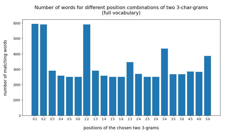
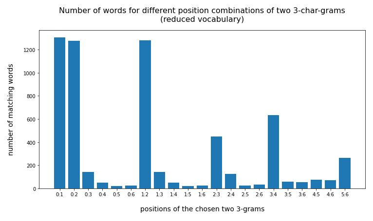
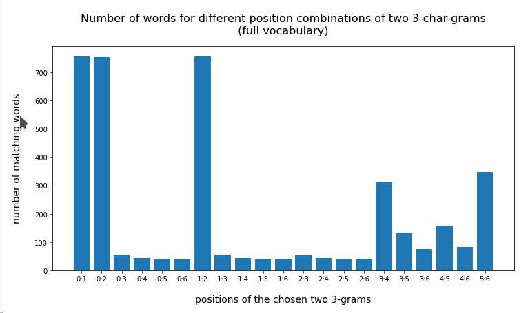
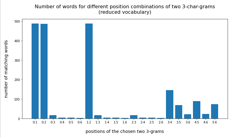
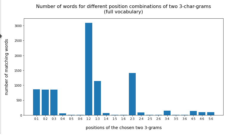
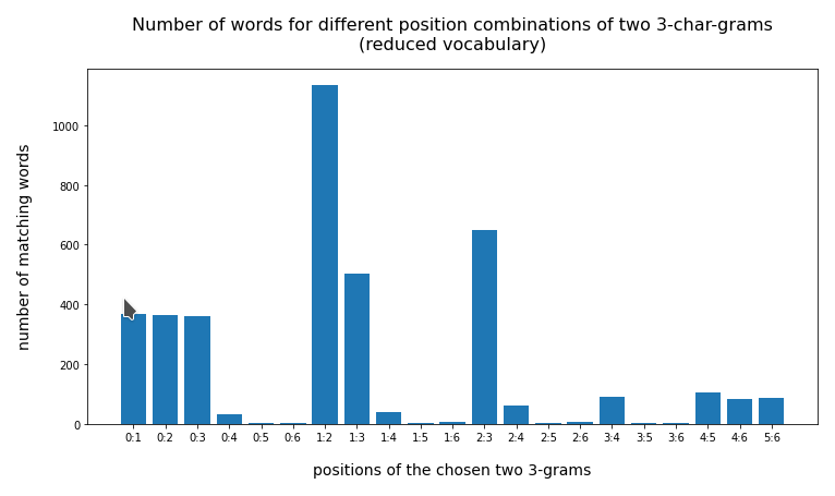
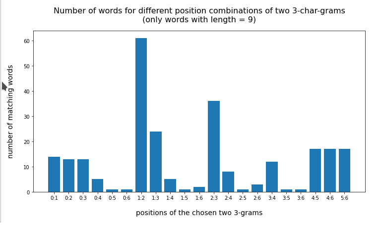
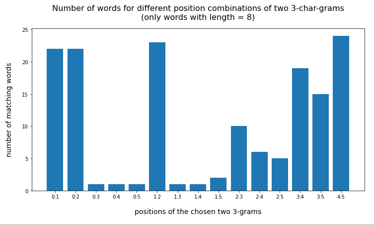
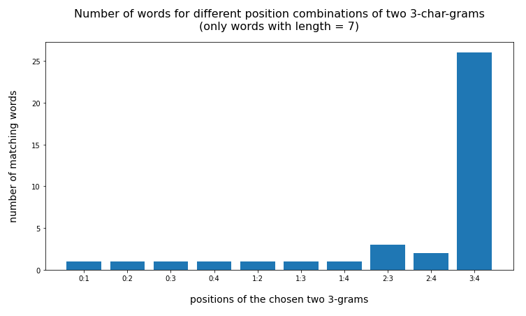
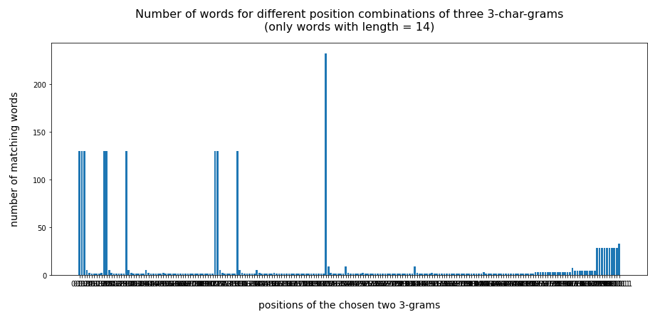
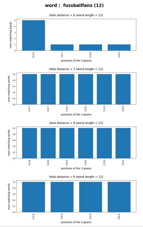
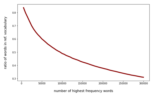
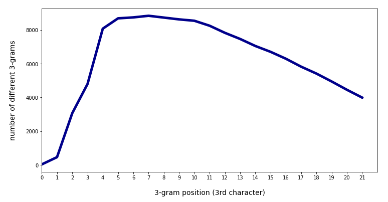
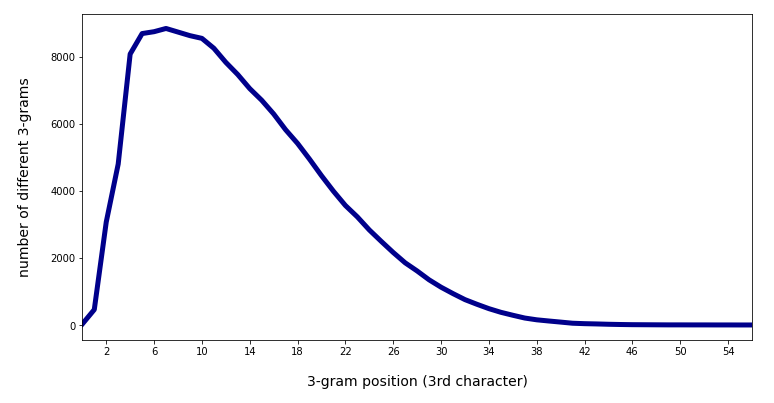
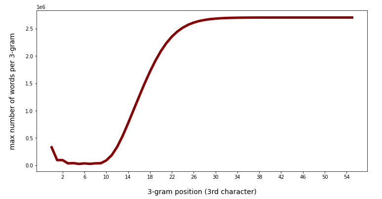
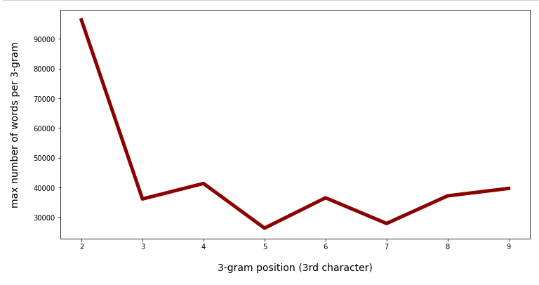
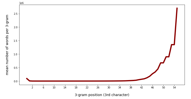
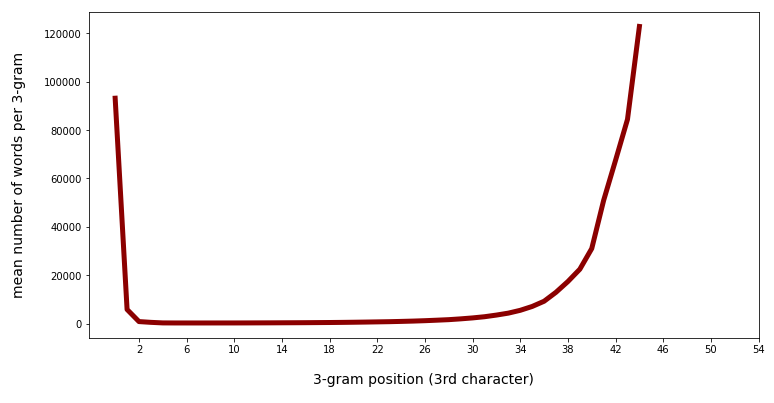
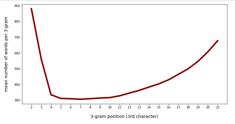
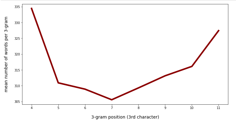
In the first post we looked at general properties of a representative German vocabulary with respect to the distribution of 3-char-gram against their position in words. In my last post we learned from some experiments that we should use 3-char-grams with some positional distance between them. This will reduce the number of matching vocabulary words to a relatively small value – mostly below 10, often even below 5. Such a small number allows for a detailed analysis of the words. The analysis for selecting the best match may, among other more complicated things, involve a character to character comparison with the original string token or a distance measure in some word vector space.

My vocabulary resides in a Pandas dataframe. Pandas is often used as a RAM based data container in the context of text analysis tasks or data preparation for machine learning. In the present article I focus on the CPU-time required to find matching vocabulary words for 100,000 different tokens with the help of two or three selected 3-char-grams. So, this is basically about the CPU-time for requests which put conditions on a few columns of a medium sized Pandas dataframe.

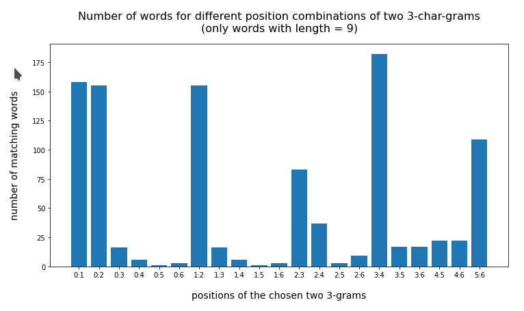
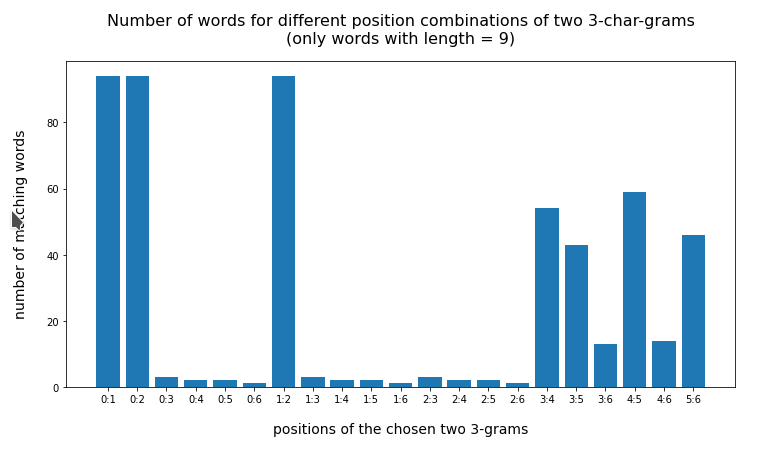
I will distinguish between searches for words with a length ≤ 9 characters and searches for longer words. Whilst processing the data I will also calculate the resulting average number of words in the hit list of matching words.

A simplifying approach

As test-tokens I pick 100,000 randomly distributed words out of my alphabetically sorted vocabulary or 100,000 words out of certain regions of the vocabulary,

I select two or three 3-char-grams out of each of these words,

I search for matching words in the vocabulary with the same 3-char-grams at their given positions within the respective word string.

So, our 3-char-grams for comparison are correctly written. In real data analysis experiments for string tokens of a given text collection the situation may be different – just wait for future posts. You may then have to vary the 3-char-gram positions to get a hit list at all. But even for correct 3-grams we already know from previous experiments that the hit list, understandably, often enough contains more than just one word.

For words ≤ 9 letters we use two 3-char-grams, for longer words three 3-char-grams. We process 7 runs in each case. The runs are different
regarding the choice of the 3-char-grams’ positions within the tokens; see the code in the sections below for the differences in the positions.

My selections of the positions of the 3-char-grams within the word follow mainly the strategy of relatively big distances between the 3-char-grams. This strategy was the main result of the last post. We also follow another insight which we got there:
For each token we use the length information, i.e. we work on a pre-defined slice of the dataframe containing only words of the same length as the token. (In the case of real life tokens you may have to vary the length parameters for different search attempts if you have reason to assume that the token is misspelled.)

I perform all test runs on a relatively old i7-6700K CPU.

Predefined slices of the vocabulary for words with a given length

We first create slices for words of a certain length and put the addresses into a dictionary:

# Create vocab slices for all word-lengths  
# ~~~~~~~~~~~~~~~~~~~~~~~~~~~--------------
b_exact_len = True

li_min = []
li_df = []
d_df  = {}
for i in range(4,57): 
    li_min.append(i)

len_li = len(li_min)
for i in range(0, len_li-1):
    mil = li_min[i]
    if b_exact_len: 
        df_x = dfw_uml.loc[(dfw_uml['len'] == mil)]
        df_x = df_x.iloc[:, 2:]
        li_df.append(df_x)
        key = "df_" + str(mil)
        d_df[key] = df_x
    else: 
        mal = li_min[i+1]
        df_x = dfw_uml.loc[(dfw_uml['len'] >= mil) & (dfw_uml['len']< mal)]
        df_x = df_x.iloc[:, 2:]
        li_df.append(df_x)
        key = "df_" + str(mil) + str(mal -1)
        d_df[key] = df_x
print("Fertig: len(li_df) = ", len(li_df), " : len(d_df) = ", len(d_df))
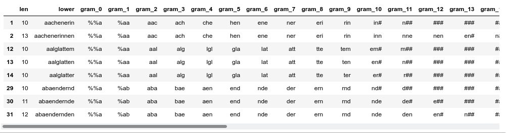
li_df[12].head(5)

Giving e.g:

Dataframe with words longer than 9 letters

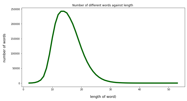
We then create a sub-dataframe containing words with “10 ≤ word-length < 30“. Reason: We know from a previous post that this selection covers most of the longer words in the vocabulary.

 
#******************************************************
# Reduce the vocab to strings in a certain length range 
# => Build dfw_short3 for long words and dfw_short2 for short words 
#******************************************************
# we produce two dfw_short frames: 
# - one for words with length >= 10  => 3-char-grams
# - one for words with length <= 9   => 2-char-grams 

# Parameters
# ~~~~~~~~~~~
min_3_len = 10
max_3_len = 30

min_2_len = 4
max_2_len = 9

mil_3 = min_3_len - 1 
mal_3 = max_3_len + 1
max_3_col = max_3_len + 4
dfw_short3 = dfw_uml.loc[(dfw_uml.lower.str.len() > mil_3) & (dfw_uml.lower.str.len() < mal_3)]
dfw_short3 = dfw_short3.iloc[:, 2:max_3_col]

mil_2 = min_2_len - 1 
mal_2 = max_2_len + 1
max_2_col = max_2_len + 4
dfw_short2 = dfw_uml.loc[(dfw_uml.lower.str.len() > mil_2) & (dfw_uml.lower.str.len() < mal_2)]
dfw_short2 = dfw_short2.iloc[:, 2:max_2_col]

print(len(dfw_short3))
print()
dfw_short3.head(8)

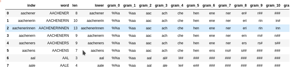
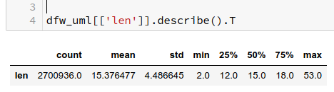
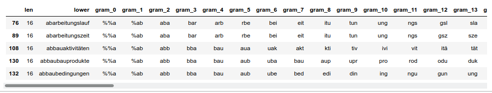
This gives us a list of around 2.5 million words (out of 2.7 million) in “dfw_short3”. The columns are “len” (containing the length), lower (containing the lower case version of a word) and columns for 3-char-grams from position 0 to 29:

nThe first 3-char-gram residing completely within the word is at column “gram_2”. We have used left- and right-padding 3-char-grams; see a previous post for this point.

The corresponding “dfw_short2” for words with a length below 10 characters is much shorter; it contains around 186000 words only.

A function to get a hit list of words matching two or three 3-char-grams

For our experiment I use the following (quick and dirty) function get_fit_words_3_grams() to select the right slice of the vocabulary and perform the search for words matching three 3-char-grams of longer string tokens:

def get_fit_words_3_grams(dfw, len_w, j, pos_l=-1, pos_m=-1, pos_r=-1, b_std_pos = True):
    # dfw: source df for tokens)
    # j: row position of token in dfw (not index-label)
    
    b_analysis = False
        
    try:
        dfw
    except NameError:
        print("dfw not defined ")
    
    # get token length 
    #len_w = dfw.iat[j,0]
    #word  = dfw.iat[j, 1]
    
    # get the right slice of the vocabulary with words corresponding to the length
    df_name = "df_" + str(len_w)
    df_ = d_df[df_name]
    
    if b_std_pos:
        j_l  = 2
        j_m  = math.floor(len_w/2)+1
        j_r  = len_w - 1 
        j_rm = j_m + 2 
    else:
        if pos_l==-1 or pos_m == -1 or pos_r == -1 or pos_m >= pos_r: 
            print("one or all of the positions is not defined or pos_m >= pos_r")
            sys.exit()
        j_l = pos_l
        j_m = pos_m
        j_r = pos_r
        if pos_m >= len_w+1 or pos_r >= len_w+2:
            print("Positions exceed defined positions of 3-char-grams for the token (len= ", len_w, ")") 
            sys.exit()

    col_l  = 'gram_' + str(j_l);  val_l  = dfw.iat[j, j_l+2]
    col_m  = 'gram_' + str(j_m);  val_m  = dfw.iat[j, j_m+2]
    col_r  = 'gram_' + str(j_r);  val_r  = dfw.iat[j, j_r+2]
    #print(len_w, ":", word, ":", j_l, ":", j_m, ":", j_r, ":", val_l, ":", val_m, ":", val_r )

    li_ind = df_.index[  (df_[col_r]==val_r) 
                       #& (df_[col_rm]==val_rm) 
                       & (df_[col_m]==val_m)
                       & (df_[col_l]==val_l)
                      ].to_list()
    
    if b_analysis:
        leng_li = len(li_ind)
        if leng_li >90:
            print("!!!!")
            for m in range(0, leng_li):
                print(df_.loc[li_ind[m], 'lower'])
            print("!!!!")
        
    #print(word, ":", leng_li, ":", len_w, ":", j_l, ":", j_m, ":", j_r, ":", val_l, ":", val_m, ":", val_r)
    return len(li_ind), len_w

For “b_std_pos == True” all 3-char-grams reside completely within the word with a maximum distance to each other.

An analogous function “get_fit_words_2_grams(dfw, len_w, j, pos_l=-1, pos_r=-1, b_std_pos = True)” basically does the same but for a chosen left and a right positioned 3-char-gram, only. The latter function is to be applied for words with a length ≤ 9.

Function to perform the test runs

A quick and dirty function to perform the planned different test runs is

# Check for 100,000 words, how long the index list is for conditions on three 3-gram_cols or two 3-grams 
# ~~~~~~~~~~~~~~~~~~~~~~~~~~~~~~~~~~~~~~~~~~~~~~~~~~~~~~~~

#Three 3-char-grams or two 3-char-grams? 
b_3 = True

# parameter
num_w   = 100000
#num_w   = 50000
n_start = 0
n_end   = n_start + num_w 

# run type 
b_random = True
pos_type = 0 
#pos_type = 1 
#pos_type = 2 
#pos_type = 3 
#pos_type = 4 
#pos_type = 5
#pos_type = 6
#pos_type = 7

if b_3: 
    len_
dfw = len(dfw_short3)
else:
    len_dfw = len(dfw_short2)
    print("len dfw_short2 = ", len_dfw)
    
if b_random: 
    random.seed()
    li_ind_w = random.sample(range(0, len_dfw), num_w)
else: 
    li_ind_w = list(range(n_start, n_end, 1))
    
#print(li_ind_w) 

if n_start+num_w > len_dfw:
    print("Error: wrong choice of params ")
    sys.exit

ay_inter_lilen = np.zeros((num_w,), dtype=np.int16)
ay_inter_wolen = np.zeros((num_w,), dtype=np.int16)

v_start_time = time.perf_counter()
n = 0 
for i in range(0, num_w):
    ind = li_ind_w[i]
    if b_3:
        leng_w = dfw_short3.iat[ind,0]
    else:
        leng_w = dfw_short2.iat[ind,0]
        
    #print(ind, leng_w)
    
    # adapt pos_l, pos_m, pos_r
    # ************************
    if pos_type == 1:
        pos_l = 3
        pos_m = math.floor(leng_w/2)+1
        pos_r = leng_w - 1
    elif pos_type == 2:
        pos_l = 2
        pos_m = math.floor(leng_w/2)+1
        pos_r = leng_w - 2
    elif pos_type == 3:
        pos_l = 4
        pos_m = math.floor(leng_w/2)+2
        pos_r = leng_w - 1
    elif pos_type == 4:
        pos_l = 2
        pos_m = math.floor(leng_w/2)
        pos_r = leng_w - 3
    elif pos_type == 5:
        pos_l = 5
        pos_m = math.floor(leng_w/2)+2
        pos_r = leng_w - 1
    elif pos_type == 6:
        pos_l = 2
        pos_m = math.floor(leng_w/2)
        pos_r = leng_w - 4
    elif pos_type == 7:
        pos_l = 3
        pos_m = math.floor(leng_w/2)
        pos_r = leng_w - 2
   
    # 3-gram check 
    if b_3:
        if pos_type == 0: 
            leng, lenw = get_fit_words_3_grams(dfw_short3, leng_w, ind, 0, 0, 0, True)
        else: 
            leng, lenw = get_fit_words_3_grams(dfw_short3, leng_w, ind, pos_l, pos_m, pos_r, False)
    else:
        if pos_type == 0: 
            leng, lenw = get_fit_words_2_grams(dfw_short2, leng_w, ind, 0, 0, True)
        else: 
            leng, lenw = get_fit_words_2_grams(dfw_short2, leng_w, ind, pos_l, pos_r, False)
    
    
    ay_inter_lilen[n] = leng
    ay_inter_wolen[n] = lenw
    #print (leng)
    n += 1
v_end_time = time.perf_counter()

cpu_time   = v_end_time - v_start_time
num_tokens = len(ay_inter_lilen)
mean_hits  = ay_inter_lilen.mean()
max_hits   = ay_inter_lilen.max()

if b_random:
    print("cpu : ", "{:.2f}".format(cpu_time), " :: tokens =", num_tokens, 
          " :: mean =", "{:.2f}".format(mean_hits), ":: max =", "{:.2f}".format(max_hits) )
else:
    print("n_start =", n_start, " :: cpu : ", "{:.2f}".format(cpu_time), ":: tokens =", num_tokens, 
      ":: mean =", "{:.2f}".format(mean_hits), ":: max =", "{:.2f}".format(max_hits) )
print()
print(ay_inter_lilen)

Test runs for words with a length ≥ 10 and three 3-char-grams

Pandas runs per default on just one CPU core. Typical run times are around 76 secs depending a bit on the background load on my Linux PC. Outputs for 3 consecutive runs for “b_random = True” runs and different “pos_type”-values and are

“b_random = True” and “pos_type = 0”

     
cpu :  75.82  :: tokens = 100000  :: mean = 1.25 :: max = 91.00
cpu :  75.40  :: tokens = 100000  :: mean = 1.25 :: max = 91.00
cpu :  75.43  :: tokens = 100000  :: mean = 1.25 :: max = 91.00

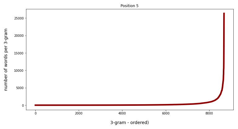
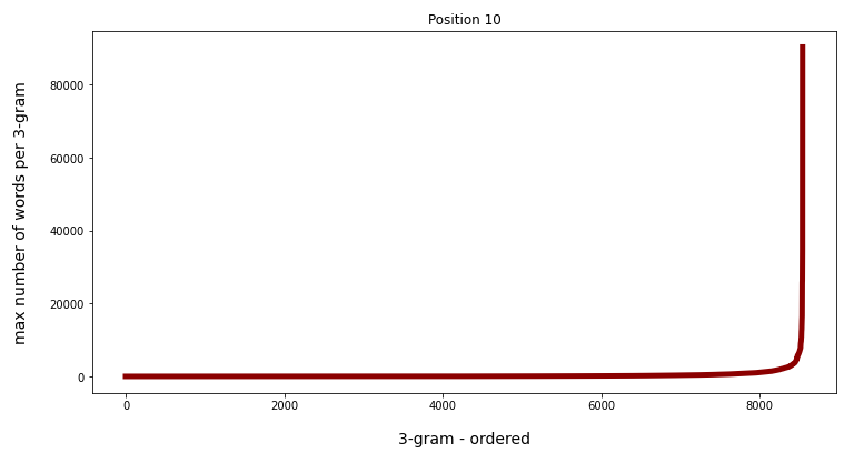
The average value “mean” for the length of the hit list is quite small. But there obviously are a few tokens for which the hit list is quite long (max-value > 90). We shall see below that the surprisingly large value of the maximum is only due to words in two specific regions of the vocabulary.

The next section for “pos_type = 1” shows a better behavior:

“b_random = True” and “pos_type = 1”
n

cpu :  75.23  :: tokens = 100000  :: mean = 1.18 :: max = 27.00
cpu :  76.39  :: tokens = 100000  :: mean = 1.18 :: max = 24.00
cpu :  75.95  :: tokens = 100000  :: mean = 1.17 :: max = 27.00

The next position variation again suffers from words in the same regions of the vocabulary where we got problems already for pos_type = 0:

“b_random = True” and “pos_type = 2”

cpu :  75.07  :: tokens = 100000  :: mean = 1.28 :: max = 52.00
cpu :  75.57  :: tokens = 100000  :: mean = 1.28 :: max = 52.00
cpu :  75.78  :: tokens = 100000  :: mean = 1.28 :: max = 52.00

The next positional variation shows a much lower max-value; the mean value is convincing:

“b_random = True” and “pos_type = 3”

cpu :  74.70  :: tokens = 100000  :: mean = 1.21 :: max = 23.00
cpu :  74.78  :: tokens = 100000  :: mean = 1.22 :: max = 23.00
cpu :  74.48  :: tokens = 100000  :: mean = 1.22 :: max = 24.00

“b_random = True” and “pos_type = 4”

cpu :  75.18  :: tokens = 100000  :: mean = 1.27 :: max = 52.00
cpu :  75.45  :: tokens = 100000  :: mean = 1.26 :: max = 52.00
cpu :  74.65  :: tokens = 100000  :: mean = 1.27 :: max = 52.00

For “pos_type = 5” we get again worse results for the average values:

“b_random = True” and “pos_type = 5”

cpu :  74.21  :: tokens = 100000  :: mean = 1.70 :: max = 49.00
cpu :  74.95  :: tokens = 100000  :: mean = 1.71 :: max = 49.00
cpu :  74.28  :: tokens = 100000  :: mean = 1.70 :: max = 49.00

“b_random = True” and “pos_type = 6”

cpu :  74.21  :: tokens = 100000  :: mean = 1.49 :: max = 31.00
cpu :  74.16  :: tokens = 100000  :: mean = 1.49 :: max = 28.00
cpu :  74.21  :: tokens = 100000  :: mean = 1.50 :: max = 31.00

“b_random = True” and “pos_type = 7”

cpu :  75.02  :: tokens = 100000  :: mean = 1.28 :: max = 34.00
cpu :  74.19  :: tokens = 100000  :: mean = 1.28 :: max = 34.00
cpu :  73.56  :: tokens = 100000  :: mean = 1.28 :: max = 34.00

The data for the mean number of matching words are overall consistent with our general considerations and observations in the previous post of this article series. The CPU-times are very reasonable – even if we had to perform 5 different 3-char-gram requests per token we could do this within 6,5 to 7 minutes.

A bit worrying is the result for the maximum of the hit-list length. The next section will show that the max-values above stem from some words in two distinct sections of the vocabulary.

Data for certain regions of the vocabulary

It is always reasonable to look a bit closer at different regions of the vocabulary. Therefore, we repeat some runs – but this time not for random data, but for 100,000 tokens following a certain start-position in the alphabetically sorted vocabulary:

“b_random = False” and “pos_type = 0” and num_w = 50,000

n_start = 0       :: tokens = 50000 :: mean = 1.10 :: max = 10
n_start = 50000   :: tokens = 50000 :: mean = 1.15 :: max = 14
n_start = 100000  :: tokens = 50000 :: mean = 1.46 :: max = 26
n_start = 150000  :: tokens = 50000 :: mean = 1.25 :: max = 26
n_start = 200000  :: tokens = 50000 :: mean = 1.30 :: max = 14
n_start = 250000  :: tokens = 50000 :: mean = 1.15 :: max = 20
n_start = 300000  :: tokens = 50000 :: mean = 1.10 :: max = 13
n_start = 350000  :: tokens = 50000 :: mean = 1.07 :: max = 6
n_start = 400000  :: tokens = 50000 :: mean = 1.11 :: max = 12
n_start = 450000  :: tokens = 50000 :: mean = 1.28 :: max = 14
n_start = 500000  :: tokens = 50000 :: mean = 1.38 :: max = 20
n_start = 550000  :: tokens = 50000 :: mean = 1.12 :: max = 15
n_start = 600000  :: tokens = 50000 :: mean = 1.
11 :: max = 11
n_start = 650000  :: tokens = 50000 :: mean = 1.18 :: max = 16
n_start = 700000  :: tokens = 50000 :: mean = 1.12 :: max = 17
n_start = 750000  :: tokens = 50000 :: mean = 1.20 :: max = 19
n_start = 800000  :: tokens = 50000 :: mean = 1.32 :: max = 21
n_start = 850000  :: tokens = 50000 :: mean = 1.13 :: max = 13
n_start = 900000  :: tokens = 50000 :: mean = 1.11 :: max = 9
n_start = 950000  :: tokens = 50000 :: mean = 1.15 :: max = 14
n_start = 1000000 :: tokens = 50000 :: mean = 1.21 :: max = 25
n_start = 1050000 :: tokens = 50000 :: mean = 1.08 :: max = 7
n_start = 1100000 :: tokens = 50000 :: mean = 1.08 :: max = 10
n_start = 1150000 :: tokens = 50000 :: mean = 1.32 :: max = 20
n_start = 1200000 :: tokens = 50000 :: mean = 1.14 :: max = 18
n_start = 1250000 :: tokens = 50000 :: mean = 1.15 :: max = 14
n_start = 1300000 :: tokens = 50000 :: mean = 1.10 :: max = 12
n_start = 1350000 :: tokens = 50000 :: mean = 1.14 :: max = 13
n_start = 1400000 :: tokens = 50000 :: mean = 1.09 :: max = 11
n_start = 1450000 :: tokens = 50000 :: mean = 1.12 :: max = 12
n_start = 1500000 :: tokens = 50000 :: mean = 1.15 :: max = 33
n_start = 1550000 :: tokens = 50000 :: mean = 1.15 :: max = 19
n_start = 1600000 :: tokens = 50000 :: mean = 1.27 :: max = 28
n_start = 1650000 :: tokens = 50000 :: mean = 1.10 :: max = 11
n_start = 1700000 :: tokens = 50000 :: mean = 1.13 :: max = 15
n_start = 1750000 :: tokens = 50000 :: mean = 1.23 :: max = 57
n_start = 1800000 :: tokens = 50000 :: mean = 1.79 :: max = 57
n_start = 1850000 :: tokens = 50000 :: mean = 1.44 :: max = 57
n_start = 1900000 :: tokens = 50000 :: mean = 1.17 :: max = 20
n_start = 1950000 :: tokens = 50000 :: mean = 1.24 :: max = 19
n_start = 2000000 :: tokens = 50000 :: mean = 1.31 :: max = 19
n_start = 2050000 :: tokens = 50000 :: mean = 1.08 :: max = 19
n_start = 2100000 :: tokens = 50000 :: mean = 1.12 :: max = 17
n_start = 2150000 :: tokens = 50000 :: mean = 1.24 :: max = 27
n_start = 2200000 :: tokens = 50000 :: mean = 2.39 :: max = 91
n_start = 2250000 :: tokens = 50000 :: mean = 2.76 :: max = 91
n_start = 2300000 :: tokens = 50000 :: mean = 1.14 :: max = 10
n_start = 2350000 :: tokens = 50000 :: mean = 1.17 :: max = 12
n_start = 2400000 :: tokens = 50000 :: mean = 1.18 :: max = 21
n_start = 2450000 :: tokens = 50000 :: mean = 1.16 :: max = 24

These data are pretty consistent with the random approach. We see that there are some intervals were the hit list gets bigger – but on average not bigger than 3.

However, we learn something important here:

In all segments of the vocabulary there are some relatively few words for which our recipe of distanced 3-car-grams nevertheless leads to long hit lists.

This is also reflected by the data for other positional distributions of the 3-char-grams:

“b_random = False” and “pos_type = 1” and num_w = 50,000

n_start = 0       :: tokens = 50000 :: mean = 1.08 :: max = 10
n_start = 50000   :: tokens = 50000 :: mean = 1.14 :: max = 14
n_start = 100000  :: tokens = 50000 :: mean = 1.16 :: max = 13
n_start = 150000  :: tokens = 50000 :: mean = 1.17 :: max = 16
n_start = 200000  :: tokens = 50000 :: mean = 1.24 :: max = 15
n_start = 250000  :: tokens = 50000 :: mean = 1.15 :: max = 20
n_start = 300000  :: tokens = 50000 :: mean = 1.12 :: max = 12
n_start = 350000  :: tokens = 50000 :: mean = 1.13 :: max = 13
n_start = 400000  :: tokens = 50000 :: mean = 1.13 :: max = 18
n_start = 450000  :: tokens = 50000 :: mean = 1.12 :: max = 10
n_start = 500000  :: tokens = 50000 :: mean = 1.20 :: max = 18
n_start = 550000  :: tokens = 50000 :: mean = 1.15 :: max = 19
n_start = 600000  :: tokens = 50000 :: mean = 1.13 :: max = 14
n_start = 650000  :: tokens = 50000 :: 
mean = 1.17 :: max = 18
n_start = 700000  :: tokens = 50000 :: mean = 1.15 :: max = 12
n_start = 750000  :: tokens = 50000 :: mean = 1.20 :: max = 16
n_start = 800000  :: tokens = 50000 :: mean = 1.30 :: max = 21
n_start = 850000  :: tokens = 50000 :: mean = 1.13 :: max = 13
n_start = 900000  :: tokens = 50000 :: mean = 1.14 :: max = 13
n_start = 950000  :: tokens = 50000 :: mean = 1.16 :: max = 14
n_start = 1000000 :: tokens = 50000 :: mean = 1.22 :: max = 25
n_start = 1050000 :: tokens = 50000 :: mean = 1.12 :: max = 14
n_start = 1100000 :: tokens = 50000 :: mean = 1.11 :: max = 12
n_start = 1150000 :: tokens = 50000 :: mean = 1.24 :: max = 16
n_start = 1200000 :: tokens = 50000 :: mean = 1.14 :: max = 18
n_start = 1250000 :: tokens = 50000 :: mean = 1.25 :: max = 15
n_start = 1300000 :: tokens = 50000 :: mean = 1.16 :: max = 15
n_start = 1350000 :: tokens = 50000 :: mean = 1.17 :: max = 14
n_start = 1400000 :: tokens = 50000 :: mean = 1.10 :: max = 10
n_start = 1450000 :: tokens = 50000 :: mean = 1.16 :: max = 21
n_start = 1500000 :: tokens = 50000 :: mean = 1.18 :: max = 33
n_start = 1550000 :: tokens = 50000 :: mean = 1.17 :: max = 20
n_start = 1600000 :: tokens = 50000 :: mean = 1.15 :: max = 14
n_start = 1650000 :: tokens = 50000 :: mean = 1.16 :: max = 12
n_start = 1700000 :: tokens = 50000 :: mean = 1.17 :: max = 15
n_start = 1750000 :: tokens = 50000 :: mean = 1.16 :: max = 12
n_start = 1800000 :: tokens = 50000 :: mean = 1.20 :: max = 14
n_start = 1850000 :: tokens = 50000 :: mean = 1.17 :: max = 13
n_start = 1900000 :: tokens = 50000 :: mean = 1.17 :: max = 20
n_start = 1950000 :: tokens = 50000 :: mean = 1.07 :: max = 11
n_start = 2000000 :: tokens = 50000 :: mean = 1.13 :: max = 15
n_start = 2050000 :: tokens = 50000 :: mean = 1.10 :: max = 8
n_start = 2100000 :: tokens = 50000 :: mean = 1.15 :: max = 17
n_start = 2150000 :: tokens = 50000 :: mean = 1.27 :: max = 27
n_start = 2200000 :: tokens = 50000 :: mean = 1.47 :: max = 24
n_start = 2250000 :: tokens = 50000 :: mean = 1.34 :: max = 22
n_start = 2300000 :: tokens = 50000 :: mean = 1.18 :: max = 12
n_start = 2350000 :: tokens = 50000 :: mean = 1.19 :: max = 14
n_start = 2400000 :: tokens = 50000 :: mean = 1.25 :: max = 21
n_start = 2450000 :: tokens = 50000 :: mean = 1.17 :: max = 25

“b_random = False” and “pos_type = 2” and num_w = 50,000

n_start = 0       :: tokens = 50000 :: mean = 1.25 :: max = 11
n_start = 50000   :: tokens = 50000 :: mean = 1.25 :: max = 8
n_start = 100000  :: tokens = 50000 :: mean = 1.50 :: max = 18
n_start = 150000  :: tokens = 50000 :: mean = 1.25 :: max = 18
n_start = 200000  :: tokens = 50000 :: mean = 1.36 :: max = 15
n_start = 250000  :: tokens = 50000 :: mean = 1.19 :: max = 13
n_start = 300000  :: tokens = 50000 :: mean = 1.15 :: max = 7
n_start = 350000  :: tokens = 50000 :: mean = 1.15 :: max = 6
n_start = 400000  :: tokens = 50000 :: mean = 1.18 :: max = 9
n_start = 450000  :: tokens = 50000 :: mean = 1.36 :: max = 15
n_start = 500000  :: tokens = 50000 :: mean = 1.39 :: max = 14
n_start = 550000  :: tokens = 50000 :: mean = 1.20 :: max = 15
n_start = 600000  :: tokens = 50000 :: mean = 1.16 :: max = 6
n_start = 650000  :: tokens = 50000 :: mean = 1.21 :: max = 8
n_start = 700000  :: tokens = 50000 :: mean = 1.18 :: max = 8
n_start = 750000  :: tokens = 50000 :: mean = 1.27 :: max = 12
n_start = 800000  :: tokens = 50000 :: mean = 1.32 :: max = 13
n_start = 850000  :: tokens = 50000 :: mean = 1.18 :: max = 8
n_start = 900000  :: tokens = 50000 :: mean = 1.17 :: max = 8
n_start = 950000  :: tokens = 50000 :: mean = 1.25 :: max = 10
n_start = 1000000 :: tokens = 50000 :: mean = 1.22 :: max = 11
n_start = 1050000 :: tokens = 50000 :: mean = 1.15 :: max = 8
n_start = 1100000 :: tokens = 50000 :: mean = 1.15 :: max = 6
r
n_start = 1150000 :: tokens = 50000 :: mean = 1.29 :: max = 15
n_start = 1200000 :: tokens = 50000 :: mean = 1.17 :: max = 7
n_start = 1250000 :: tokens = 50000 :: mean = 1.17 :: max = 8
n_start = 1300000 :: tokens = 50000 :: mean = 1.16 :: max = 9
n_start = 1350000 :: tokens = 50000 :: mean = 1.18 :: max = 8
n_start = 1400000 :: tokens = 50000 :: mean = 1.17 :: max = 8
n_start = 1450000 :: tokens = 50000 :: mean = 1.17 :: max = 7
n_start = 1500000 :: tokens = 50000 :: mean = 1.17 :: max = 9
n_start = 1550000 :: tokens = 50000 :: mean = 1.17 :: max = 7
n_start = 1600000 :: tokens = 50000 :: mean = 1.31 :: max = 24
n_start = 1650000 :: tokens = 50000 :: mean = 1.18 :: max = 9
n_start = 1700000 :: tokens = 50000 :: mean = 1.17 :: max = 13
n_start = 1750000 :: tokens = 50000 :: mean = 1.26 :: max = 21
n_start = 1800000 :: tokens = 50000 :: mean = 1.70 :: max = 21
n_start = 1850000 :: tokens = 50000 :: mean = 1.43 :: max = 21
n_start = 1900000 :: tokens = 50000 :: mean = 1.19 :: max = 10
n_start = 1950000 :: tokens = 50000 :: mean = 1.30 :: max = 11
n_start = 2000000 :: tokens = 50000 :: mean = 1.33 :: max = 11
n_start = 2050000 :: tokens = 50000 :: mean = 1.16 :: max = 8
n_start = 2100000 :: tokens = 50000 :: mean = 1.17 :: max = 9
n_start = 2150000 :: tokens = 50000 :: mean = 1.41 :: max = 20
n_start = 2200000 :: tokens = 50000 :: mean = 2.08 :: max = 52
n_start = 2250000 :: tokens = 50000 :: mean = 2.27 :: max = 52
n_start = 2300000 :: tokens = 50000 :: mean = 1.21 :: max = 11
n_start = 2350000 :: tokens = 50000 :: mean = 1.21 :: max = 10
n_start = 2400000 :: tokens = 50000 :: mean = 1.21 :: max = 9
n_start = 2450000 :: tokens = 50000 :: mean = 1.30 :: max = 18

“b_random = False” and “pos_type = 3” and num_w = 50,000

n_start = 0       :: tokens = 50000 :: mean = 1.23 :: max = 23
n_start = 50000   :: tokens = 50000 :: mean = 1.25 :: max = 17
n_start = 100000  :: tokens = 50000 :: mean = 1.16 :: max = 17
n_start = 150000  :: tokens = 50000 :: mean = 1.22 :: max = 15
n_start = 200000  :: tokens = 50000 :: mean = 1.22 :: max = 17
n_start = 250000  :: tokens = 50000 :: mean = 1.18 :: max = 11
n_start = 300000  :: tokens = 50000 :: mean = 1.27 :: max = 23
n_start = 350000  :: tokens = 50000 :: mean = 1.29 :: max = 23
n_start = 400000  :: tokens = 50000 :: mean = 1.14 :: max = 11
n_start = 450000  :: tokens = 50000 :: mean = 1.18 :: max = 17
n_start = 500000  :: tokens = 50000 :: mean = 1.16 :: max = 15
n_start = 550000  :: tokens = 50000 :: mean = 1.26 :: max = 17
n_start = 600000  :: tokens = 50000 :: mean = 1.20 :: max = 13
n_start = 650000  :: tokens = 50000 :: mean = 1.10 :: max = 9
n_start = 700000  :: tokens = 50000 :: mean = 1.20 :: max = 17
n_start = 750000  :: tokens = 50000 :: mean = 1.17 :: max = 17
n_start = 800000  :: tokens = 50000 :: mean = 1.28 :: max = 19
n_start = 850000  :: tokens = 50000 :: mean = 1.15 :: max = 15
n_start = 900000  :: tokens = 50000 :: mean = 1.19 :: max = 11
n_start = 950000  :: tokens = 50000 :: mean = 1.19 :: max = 13
n_start = 1000000 :: tokens = 50000 :: mean = 1.24 :: max = 24
n_start = 1050000 :: tokens = 50000 :: mean = 1.17 :: max = 10
n_start = 1100000 :: tokens = 50000 :: mean = 1.29 :: max = 23
n_start = 1150000 :: tokens = 50000 :: mean = 1.18 :: max = 13
n_start = 1200000 :: tokens = 50000 :: mean = 1.18 :: max = 16
n_start = 1250000 :: tokens = 50000 :: mean = 1.38 :: max = 23
n_start = 1300000 :: tokens = 50000 :: mean = 1.30 :: max = 23
n_start = 1350000 :: tokens = 50000 :: mean = 1.21 :: max = 15
n_start = 1400000 :: tokens = 50000 :: mean = 1.21 :: max = 23
n_start = 1450000 :: tokens = 50000 :: mean = 1.23 :: max = 12
n_start = 1500000 :: tokens = 50000 :: mean = 1.21 :: max = 13
n_start = 1550000 :: tokens = 50000 :: mean = 1.22 :: max = 12
n_start = 1600000 :: 
tokens = 50000 :: mean = 1.12 :: max = 13
n_start = 1650000 :: tokens = 50000 :: mean = 1.27 :: max = 16
n_start = 1700000 :: tokens = 50000 :: mean = 1.23 :: max = 15
n_start = 1750000 :: tokens = 50000 :: mean = 1.26 :: max = 11
n_start = 1800000 :: tokens = 50000 :: mean = 1.08 :: max = 7
n_start = 1850000 :: tokens = 50000 :: mean = 1.11 :: max = 12
n_start = 1900000 :: tokens = 50000 :: mean = 1.26 :: max = 23
n_start = 1950000 :: tokens = 50000 :: mean = 1.06 :: max = 9
n_start = 2000000 :: tokens = 50000 :: mean = 1.11 :: max = 15
n_start = 2050000 :: tokens = 50000 :: mean = 1.16 :: max = 16
n_start = 2100000 :: tokens = 50000 :: mean = 1.17 :: max = 13
n_start = 2150000 :: tokens = 50000 :: mean = 1.33 :: max = 16
n_start = 2200000 :: tokens = 50000 :: mean = 1.29 :: max = 24
n_start = 2250000 :: tokens = 50000 :: mean = 1.20 :: max = 17
n_start = 2300000 :: tokens = 50000 :: mean = 1.35 :: max = 17
n_start = 2350000 :: tokens = 50000 :: mean = 1.25 :: max = 12
n_start = 2400000 :: tokens = 50000 :: mean = 1.26 :: max = 16
n_start = 2450000 :: tokens = 50000 :: mean = 1.29 :: max = 13

“b_random = False” and “pos_type = 4” and num_w = 50,000

n_start = 0       :: tokens = 50000 :: mean = 1.25 :: max = 6
n_start = 50000   :: tokens = 50000 :: mean = 1.27 :: max = 9
n_start = 100000  :: tokens = 50000 :: mean = 1.43 :: max = 19
n_start = 150000  :: tokens = 50000 :: mean = 1.22 :: max = 19
n_start = 200000  :: tokens = 50000 :: mean = 1.33 :: max = 12
n_start = 250000  :: tokens = 50000 :: mean = 1.22 :: max = 7
n_start = 300000  :: tokens = 50000 :: mean = 1.17 :: max = 7
n_start = 350000  :: tokens = 50000 :: mean = 1.17 :: max = 8
n_start = 400000  :: tokens = 50000 :: mean = 1.21 :: max = 8
n_start = 450000  :: tokens = 50000 :: mean = 1.32 :: max = 12
n_start = 500000  :: tokens = 50000 :: mean = 1.36 :: max = 14
n_start = 550000  :: tokens = 50000 :: mean = 1.22 :: max = 8
n_start = 600000  :: tokens = 50000 :: mean = 1.18 :: max = 6
n_start = 650000  :: tokens = 50000 :: mean = 1.23 :: max = 8
n_start = 700000  :: tokens = 50000 :: mean = 1.21 :: max = 14
n_start = 750000  :: tokens = 50000 :: mean = 1.29 :: max = 14
n_start = 800000  :: tokens = 50000 :: mean = 1.31 :: max = 13
n_start = 850000  :: tokens = 50000 :: mean = 1.19 :: max = 13
n_start = 900000  :: tokens = 50000 :: mean = 1.17 :: max = 7
n_start = 950000  :: tokens = 50000 :: mean = 1.26 :: max = 8
n_start = 1000000 :: tokens = 50000 :: mean = 1.24 :: max = 11
n_start = 1050000 :: tokens = 50000 :: mean = 1.18 :: max = 9
n_start = 1100000 :: tokens = 50000 :: mean = 1.19 :: max = 7
n_start = 1150000 :: tokens = 50000 :: mean = 1.27 :: max = 10
n_start = 1200000 :: tokens = 50000 :: mean = 1.20 :: max = 7
n_start = 1250000 :: tokens = 50000 :: mean = 1.18 :: max = 13
n_start = 1300000 :: tokens = 50000 :: mean = 1.19 :: max = 9
n_start = 1350000 :: tokens = 50000 :: mean = 1.20 :: max = 9
n_start = 1400000 :: tokens = 50000 :: mean = 1.20 :: max = 8
n_start = 1450000 :: tokens = 50000 :: mean = 1.20 :: max = 9
n_start = 1500000 :: tokens = 50000 :: mean = 1.19 :: max = 14
n_start = 1550000 :: tokens = 50000 :: mean = 1.20 :: max = 11
n_start = 1600000 :: tokens = 50000 :: mean = 1.29 :: max = 11
n_start = 1650000 :: tokens = 50000 :: mean = 1.19 :: max = 6
n_start = 1700000 :: tokens = 50000 :: mean = 1.18 :: max = 8
n_start = 1750000 :: tokens = 50000 :: mean = 1.21 :: max = 22
n_start = 1800000 :: tokens = 50000 :: mean = 1.42 :: max = 33
n_start = 1850000 :: tokens = 50000 :: mean = 1.32 :: max = 33
n_start = 1900000 :: tokens = 50000 :: mean = 1.23 :: max = 15
n_start = 1950000 :: tokens = 50000 :: mean = 1.25 :: max = 9
n_start = 2000000 :: tokens = 50000 :: mean = 1.27 :: max = 10
n_start = 2050000 :: tokens = 50000 :: mean = 1.17 :: 
max = 10
n_start = 2100000 :: tokens = 50000 :: mean = 1.19 :: max = 9
n_start = 2150000 :: tokens = 50000 :: mean = 1.40 :: max = 16
n_start = 2200000 :: tokens = 50000 :: mean = 1.82 :: max = 52
n_start = 2250000 :: tokens = 50000 :: mean = 1.94 :: max = 52
n_start = 2300000 :: tokens = 50000 :: mean = 1.21 :: max = 9
n_start = 2350000 :: tokens = 50000 :: mean = 1.20 :: max = 7
n_start = 2400000 :: tokens = 50000 :: mean = 1.24 :: max = 7
n_start = 2450000 :: tokens = 50000 :: mean = 1.31 :: max = 16

“b_random = False” and “pos_type = 5” and num_w = 50,000

n_start = 0       :: tokens = 50000 :: mean = 1.73 :: max = 49
n_start = 50000   :: tokens = 50000 :: mean = 1.59 :: max = 49
n_start = 100000  :: tokens = 50000 :: mean = 1.91 :: max = 49
n_start = 150000  :: tokens = 50000 :: mean = 1.99 :: max = 49
n_start = 200000  :: tokens = 50000 :: mean = 1.46 :: max = 44
n_start = 250000  :: tokens = 50000 :: mean = 1.74 :: max = 49
n_start = 300000  :: tokens = 50000 :: mean = 1.94 :: max = 49
n_start = 350000  :: tokens = 50000 :: mean = 2.00 :: max = 49
n_start = 400000  :: tokens = 50000 :: mean = 1.47 :: max = 49
n_start = 450000  :: tokens = 50000 :: mean = 2.04 :: max = 49
n_start = 500000  :: tokens = 50000 :: mean = 1.80 :: max = 49
n_start = 550000  :: tokens = 50000 :: mean = 1.76 :: max = 49
n_start = 600000  :: tokens = 50000 :: mean = 1.83 :: max = 44
n_start = 650000  :: tokens = 50000 :: mean = 1.43 :: max = 44
n_start = 700000  :: tokens = 50000 :: mean = 1.77 :: max = 49
n_start = 750000  :: tokens = 50000 :: mean = 1.43 :: max = 49
n_start = 800000  :: tokens = 50000 :: mean = 1.50 :: max = 32
n_start = 850000  :: tokens = 50000 :: mean = 1.71 :: max = 44
n_start = 900000  :: tokens = 50000 :: mean = 1.68 :: max = 40
n_start = 950000  :: tokens = 50000 :: mean = 1.74 :: max = 49
n_start = 1000000 :: tokens = 50000 :: mean = 1.98 :: max = 49
n_start = 1050000 :: tokens = 50000 :: mean = 1.73 :: max = 40
n_start = 1100000 :: tokens = 50000 :: mean = 1.71 :: max = 30
n_start = 1150000 :: tokens = 50000 :: mean = 1.32 :: max = 30
n_start = 1200000 :: tokens = 50000 :: mean = 1.49 :: max = 49
n_start = 1250000 :: tokens = 50000 :: mean = 1.93 :: max = 40
n_start = 1300000 :: tokens = 50000 :: mean = 1.94 :: max = 49
n_start = 1350000 :: tokens = 50000 :: mean = 1.67 :: max = 44
n_start = 1400000 :: tokens = 50000 :: mean = 1.61 :: max = 37
n_start = 1450000 :: tokens = 50000 :: mean = 1.86 :: max = 49
n_start = 1500000 :: tokens = 50000 :: mean = 2.04 :: max = 49
n_start = 1550000 :: tokens = 50000 :: mean = 1.60 :: max = 49
n_start = 1600000 :: tokens = 50000 :: mean = 1.38 :: max = 34
n_start = 1650000 :: tokens = 50000 :: mean = 1.77 :: max = 49
n_start = 1700000 :: tokens = 50000 :: mean = 1.77 :: max = 44
n_start = 1750000 :: tokens = 50000 :: mean = 1.79 :: max = 49
n_start = 1800000 :: tokens = 50000 :: mean = 1.08 :: max = 16
n_start = 1850000 :: tokens = 50000 :: mean = 1.46 :: max = 49
n_start = 1900000 :: tokens = 50000 :: mean = 1.51 :: max = 49
n_start = 1950000 :: tokens = 50000 :: mean = 1.31 :: max = 24
n_start = 2000000 :: tokens = 50000 :: mean = 1.24 :: max = 29
n_start = 2050000 :: tokens = 50000 :: mean = 1.85 :: max = 49
n_start = 2100000 :: tokens = 50000 :: mean = 1.96 :: max = 49
n_start = 2150000 :: tokens = 50000 :: mean = 1.66 :: max = 49
n_start = 2200000 :: tokens = 50000 :: mean = 1.45 :: max = 40
n_start = 2250000 :: tokens = 50000 :: mean = 1.51 :: max = 49
n_start = 2300000 :: tokens = 50000 :: mean = 2.07 :: max = 49
n_start = 2350000 :: tokens = 50000 :: mean = 2.01 :: max = 34
n_start = 2400000 :: tokens = 50000 :: mean = 1.94 :: max = 34
n_start = 2450000 :: tokens = 50000 :: mean = 1.85 :: max = 49

pos_type = 5 shows on average
larger maximum values; this is consistent with relatively high average values for the hit list length.

“b_random = False” and “pos_type = 6” and num_w = 50,000

n_start = 0       :: tokens = 50000 :: mean = 1.38 :: max = 9
n_start = 50000   :: tokens = 50000 :: mean = 1.44 :: max = 22
n_start = 100000  :: tokens = 50000 :: mean = 1.58 :: max = 14
n_start = 150000  :: tokens = 50000 :: mean = 1.41 :: max = 20
n_start = 200000  :: tokens = 50000 :: mean = 1.51 :: max = 16
n_start = 250000  :: tokens = 50000 :: mean = 1.43 :: max = 17
n_start = 300000  :: tokens = 50000 :: mean = 1.41 :: max = 20
n_start = 350000  :: tokens = 50000 :: mean = 1.34 :: max = 17
n_start = 400000  :: tokens = 50000 :: mean = 1.47 :: max = 21
n_start = 450000  :: tokens = 50000 :: mean = 1.56 :: max = 18
n_start = 500000  :: tokens = 50000 :: mean = 1.54 :: max = 21
n_start = 550000  :: tokens = 50000 :: mean = 1.40 :: max = 22
n_start = 600000  :: tokens = 50000 :: mean = 1.41 :: max = 22
n_start = 650000  :: tokens = 50000 :: mean = 1.47 :: max = 21
n_start = 700000  :: tokens = 50000 :: mean = 1.47 :: max = 19
n_start = 750000  :: tokens = 50000 :: mean = 1.51 :: max = 21
n_start = 800000  :: tokens = 50000 :: mean = 1.51 :: max = 17
n_start = 850000  :: tokens = 50000 :: mean = 1.36 :: max = 15
n_start = 900000  :: tokens = 50000 :: mean = 1.39 :: max = 27
n_start = 950000  :: tokens = 50000 :: mean = 1.53 :: max = 22
n_start = 1000000 :: tokens = 50000 :: mean = 1.45 :: max = 22
n_start = 1050000 :: tokens = 50000 :: mean = 1.45 :: max = 16
n_start = 1100000 :: tokens = 50000 :: mean = 1.49 :: max = 31
n_start = 1150000 :: tokens = 50000 :: mean = 1.46 :: max = 31
n_start = 1200000 :: tokens = 50000 :: mean = 1.55 :: max = 20
n_start = 1250000 :: tokens = 50000 :: mean = 1.33 :: max = 14
n_start = 1300000 :: tokens = 50000 :: mean = 1.44 :: max = 27
n_start = 1350000 :: tokens = 50000 :: mean = 1.41 :: max = 16
n_start = 1400000 :: tokens = 50000 :: mean = 1.43 :: max = 19
n_start = 1450000 :: tokens = 50000 :: mean = 1.46 :: max = 20
n_start = 1500000 :: tokens = 50000 :: mean = 1.32 :: max = 15
n_start = 1550000 :: tokens = 50000 :: mean = 1.39 :: max = 18
n_start = 1600000 :: tokens = 50000 :: mean = 1.52 :: max = 20
n_start = 1650000 :: tokens = 50000 :: mean = 1.36 :: max = 17
n_start = 1700000 :: tokens = 50000 :: mean = 1.41 :: max = 17
n_start = 1750000 :: tokens = 50000 :: mean = 1.38 :: max = 19
n_start = 1800000 :: tokens = 50000 :: mean = 1.80 :: max = 20
n_start = 1850000 :: tokens = 50000 :: mean = 1.63 :: max = 25
n_start = 1900000 :: tokens = 50000 :: mean = 1.52 :: max = 21
n_start = 1950000 :: tokens = 50000 :: mean = 1.52 :: max = 22
n_start = 2000000 :: tokens = 50000 :: mean = 1.53 :: max = 25
n_start = 2050000 :: tokens = 50000 :: mean = 1.33 :: max = 14
n_start = 2100000 :: tokens = 50000 :: mean = 1.41 :: max = 23
n_start = 2150000 :: tokens = 50000 :: mean = 1.61 :: max = 19
n_start = 2200000 :: tokens = 50000 :: mean = 2.03 :: max = 28
n_start = 2250000 :: tokens = 50000 :: mean = 2.12 :: max = 28
n_start = 2300000 :: tokens = 50000 :: mean = 1.47 :: max = 26
n_start = 2350000 :: tokens = 50000 :: mean = 1.42 :: max = 21
n_start = 2400000 :: tokens = 50000 :: mean = 1.50 :: max = 21
n_start = 2450000 :: tokens = 50000 :: mean = 1.49 :: max = 22

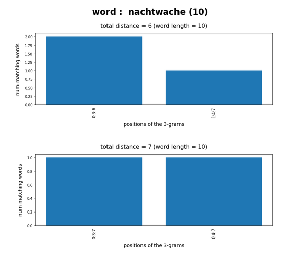
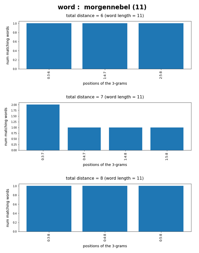
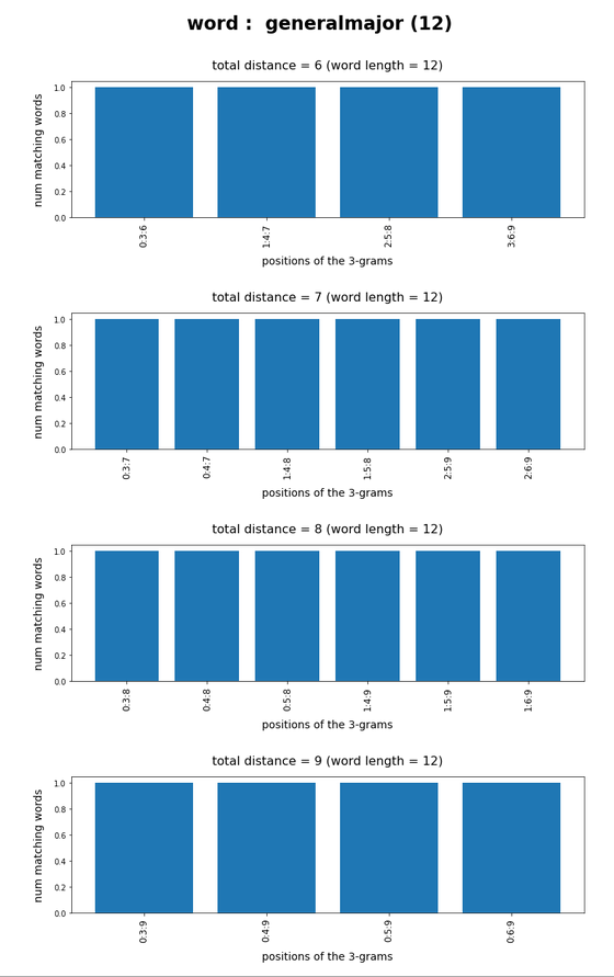
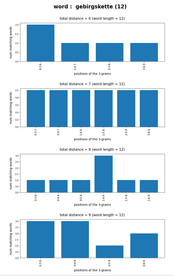
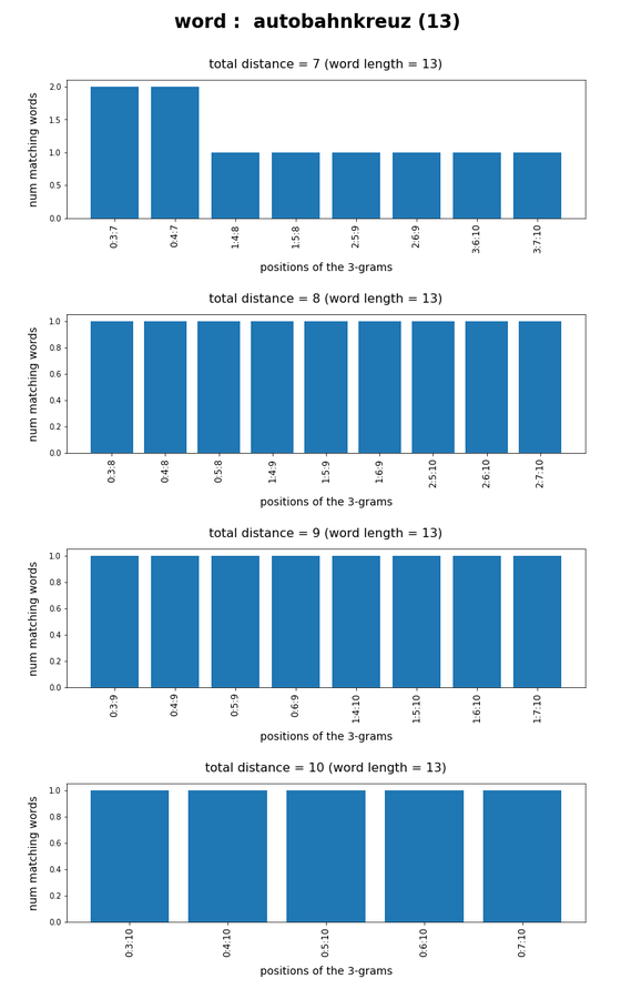
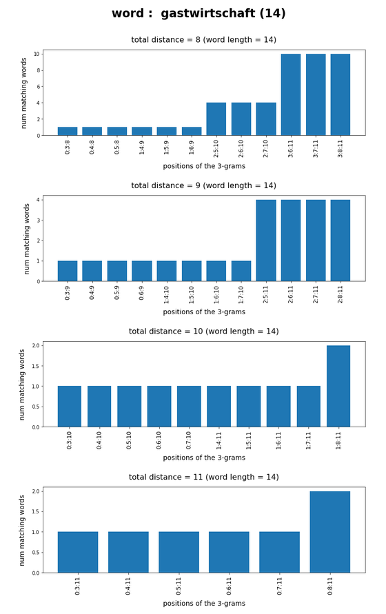
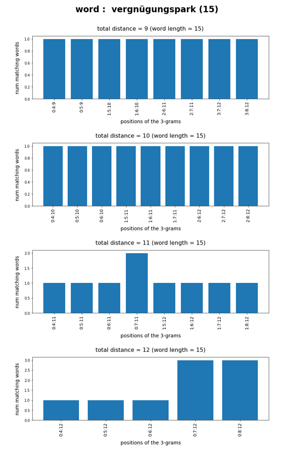
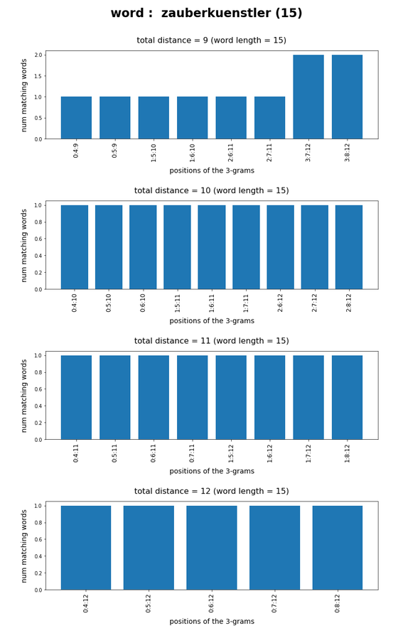
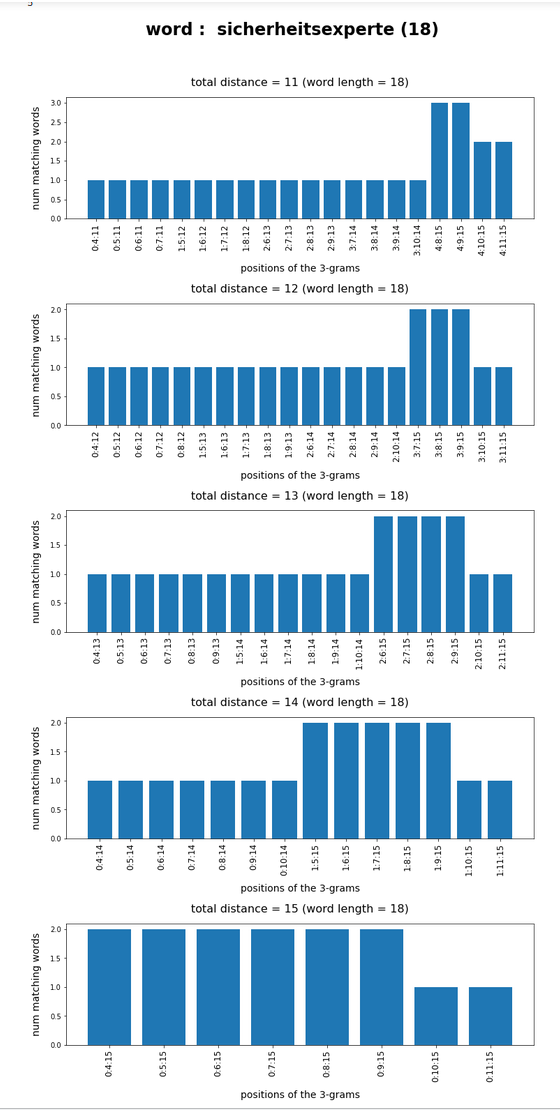
For pos_type == 0 typical examples for many hits are members of the following word collection. You see the common 3-char-grams at the beginning, in the middle and at the end of the words:

verbindungsbauten, verbindungsfesten, verbindungskanten, verbindungskarten, verbindungskasten,
verbindungsketten, verbindungsknoten, verbindungskosten, verbindungsleuten, verbindungslisten,
verbindungsmasten, verbindungspisten, verbindungsrouten, verbindungsweiten, 
verbindungszeiten,
verfassungsraeten, verfassungstexten, verfassungswerten, verfolgungslisten, verfolgungsnoeten, 
verfolgungstexten, verfolgungszeiten, verführungsküsten, vergnügungsbauten, vergnügungsbooten,
vergnügungsfesten, vergnügungsgarten, vergnügungsgärten, verguetungskosten, verletzungsnoeten, 
vermehrungsbauten, vermehrungsbeeten, vermehrungsgarten, vermessungsbooten, vermessungskarten,
vermessungsketten, vermessungskosten, vermessungslatten, vermessungsposten, vermessungsseiten,
vermietungslisten, verordnungstexten, verpackungskisten, verpackungskosten, verpackungsresten,
verpackungstexten, versorgungsbauten, versorgungsbooten, versorgungsgarten, versorgungsgärten,
versorgungshütten, versorgungskarten, versorgungsketten, versorgungskisten, versorgungsknoten,
versorgungskosten, versorgungslasten, versorgungslisten, versorgungsposten, versorgungsquoten,
versorgungsrenten, versorgungsrouten, versorgungszeiten, verteilungseliten, verteilungskarten,
verteilungskosten, verteilungslisten, verteilungsposten, verteilungswerten, vertretungskosten,
vertretungswerten, vertretungszeiten, vertretungsärzten, verwaltungsbauten, verwaltungseliten,
verwaltungskarten, verwaltungsketten, verwaltungsknoten, verwaltungskonten, verwaltungskosten, 
verwaltungslasten, verwaltungsleuten, verwaltungsposten, verwaltungsraeten, verwaltungstexten,
verwaltungsärzten, verwendungszeiten, verwertungseliten, verwertungsketten, verwertungskosten,
verwertungsquoten

For pos_type == 5 we get the following example words with many hits:

almbereich, altbereich, armbereich, astbereich, barbereich, baubereich, 
biobereich, bobbereich, boxbereich, busbereich, bußbereich, dombereich,
eckbereich, eisbereich, endbereich, erdbereich, essbereich, fußbereich,
gasbereich, genbereich, hofbereich, hubbereich, hutbereich, hörbereich,
kurbereich, lötbereich, nahbereich, oelbereich, ohrbereich, ostbereich,
radbereich, rotbereich, seebereich, sehbereich, skibereich, subbereich,
südbereich, tatbereich, tonbereich, topbereich, torbereich, totbereich,
türbereich, vorbereich, webbereich, wegbereich, zoobereich, zugbereich,
ökobereich

Intermediate conclusion for tokens longer than 9 letters

From what we found above something like “0 <= pos-type <= 4" and "pos_type =7" are preferable choices for the positions of the 3-char-grams in longer words. But even if we have to vary the positions a bit more, we get on average reasonably short hit lists.

It seems, however, that we must live with relatively long hit lists for some words (mostly compounds at a certain region of the vocabulary).

Test runs for words with a length ≤ 9 and two 3-char-grams

The list of words with less than 10 characters comprises only around 185869 entries. So, the cpu-time required should become smaller.

Here are some result data for runs for words with a length ≤ 9 characters:

“b_random = True” and “pos_type = 0”

     
cpu :  42.69  :: tokens = 100000  :: mean = 2.07 :: max = 78.00

“b_random = True” and “pos_type = 1”

cpu :  43.76  :: tokens = 100000  :: mean = 1.84 :: max = 40.00

“b_random = True” and “pos_type = 2”

cpu :  43.18  :: tokens = 100000  :: mean = 1.76 :: max = 30.00

“b_random = True” and “pos_type = 3”

cpu :  43.91  :: tokens = 100000  :: mean = 2.66 :: max = 46.00

“b_random = True” and “pos_type = 4”

cpu :  43.64  :: tokens = 100000  :: mean = 2.09 :: max = 30.00

“b_random = True” and “pos_type = 5”

cpu :  44.00  :: tokens = 100000  :: mean = 9.38 :: max = 265.00

“b_random = True” and “pos_type = 6”

cpu :  43.59  :: tokens = 100000  :: mean = 5.71 :: 
max = 102.00

“b_random = True” and “pos_type = 7”

cpu :  43.50  :: tokens = 100000  :: mean = 2.07 :: max = 30.00

You see that we should not shift the first or the last 3-char-gram to far into the middle of the word. For short tokens such a shift can lead to a full overlap of the 3-char-grams – and this obviously reduces our chances to reduce the list of hits.

Conclusion

In this post we continued our experiments on selecting words from a vocabulary which match some 3-char-grams at different positions of the token. We found the following:

The measured CPU-times for 100,000 tokens allow for multiple word searches with different positions of two or three 3-char-grams, even on a PC.
While we, on average, get hit lists of a length below 2 matching words there are always a few compounds which lead to significantly larger hit lists with tenths of words.
For tokens with a length less than 9 characters, we can work with two 3-char-grams – but we should avoid a too big overlap of the char-grams.

These results give us some hope that we can select a reasonably short list of words from a vocabulary which match parts of misspelled tokens – e.g. with one or sometimes two letters wrongly written. Before we turn to the challenge of correcting such tokens in a new article series we close the present series with yet another post about the effect of multiprocessing on our word selection processes.

Pandas dataframe, German vocabulary – select words by matching a few 3-char-grams – II

Posted on 12. September 2021 by eremo

In my last post

Pandas dataframe, German vocabulary – select words by matching a few 3-char-grams – I

I have discussed some properties of 3-char-grams of words in a German word list. (See the named post for the related structure of a Pandas dataframe (“dfw_uml”) which hosts both the word list and all corresponding 3-char-grams.) In particular I presented the distribution of the maximum and mean number of words per unique 3-char-gram against the position of the 3-char-grams inside the the words of my vocabulary.

In the present post I want to use the very same Pandas dataframe to find German words which match two or three 3-char-grams defined at different positions inside some given strings or “tokens” of a text to be analyzed by a computer. One question in such a context is: How do we choose the 3-char-gram-positions to make the selection process effective in the sense of a short list of possible hits?

The dataframe has in my case 2.7 million rows for individual words and up to 55 columns for the values 3-char-grams at 55 positions. In the case of short words the columns are filled by artificial 3-char-grams “###”.

My objective and a naive approach

Let us assume that we have a string (or “token”) of e.g. 15 characters for a (German) word. The token contains some error in the sense of a wrongly written or omitted letter. Unfortunately, our text-analysis program does not know which letter of the string is wrongly written. So it wants to find words which may fit to the general character structure. We therefore pick a few 3-grams at given positions of our token. We then want to find words which match two or three 3-char-grams at different positions of the string – hoping that we chose 3-char-grams which do not contain any error. If we get no match we try different a different combination of 3-gram-positions.

In such a brute-force comparison process you would like to quickly pin down the number of matching words with a very limited bunch of 3-grams of the test token. The grams’ positions should be chosen such that the hit list contains a minimum of fitting words. We, therefore, can pose this problem in a different way:

Which chosen positions or positional distances of two or three 3-char-grams inside a string token reduces the list of matching words from a vocabulary to a minimum?

Maybe there is a theoretically well founded solution for this problem. Personally, I am too old and too lazy to analyze such problems with solid mathematical statistics. I take a shortcut and trust my guts. It seems reasonable to me that the selected 3-char-grams should be distributed across the test string with a maximum distance between them. Let us see how far we get with this naive approach.

For the experiments discussed below I use

three 3-char-grams for tokens longer than 9 characters.
two 3-char-grams for tokens shorter than 9 letters.

For our first tests we pick correctly written 3-char-grams of test words. This means that we take correctly written words as our test tokens. The handling of tokens with wrongly written characters will be the topic of future articles.

Position combinations of two 3-char-grams for relatively short words

To get some idea about the problem’s structure I first pick a test-word like “eisenbahn”. As it is a relatively short word we start working with only two 3-char-grams. My test-word is an interesting one as it is a compound of two individual words “eisen” and “bahn”. There are many other words in the German language which either contain the first or the second word. And in German we can
add even more words to get even longer compounds. So, we would guess with some confidence that there are many hits if we chose two 3-char-grams overlapping each other or being located too close to each other. In addition we would also expect that we should use the length information about the token (or the sought words) during the selection process.

With a stride of 1 we have exactly seven 3-char-grams which reside completely inside our test-word. This gives us 21 options to use two 3-char-grams to find matching words.

To raise the chance for a bunch of alternative results we first look at words with up to 12 characters in our vocabulary and create a respective shortened slice of our dataframe “dfw_uml”:

# Reduce the vocab to strings < max_len => Build dfw_short
#*********************************
#b_exact_length = False
b_exact_length = True

min_len = 4
max_len = 12
length  = 9

mil = min_len - 1 
mal = max_len + 1

if b_exact_length: 
    dfw_short = dfw_uml.loc[(dfw_uml.lower.str.len() == length)]
else:     
    dfw_short = dfw_uml.loc[(dfw_uml.lower.str.len() > mil) & (dfw_uml.lower.str.len() < mal)]
dfw_short = dfw_short.iloc[:, 2:26]
print(len(dfw_short))
dfw_short.head(5)

The above code allows us to choose whether we shorten the vocabulary to words with a length inside an interval or to words with a defined exact length. A quick and dirty code fragment to evaluate some statistics for all possible 21 position combinations for two 3-char-grams is the following:

# Hits for two 3-grams distributed over 9-letter and shorter words
# *****************************************************************
b_full_vocab  = False # operate on the full vocabulary 
#b_full_vocab  = True # operate on the full vocabulary 

word  = "eisenbahn"
word  = "löwenzahn"
word  = "kellertür"
word  = "nashorn"
word  = "vogelart"

d_col = { "col_0": "gram_2", "col_1": "gram_3", "col_2": "gram_4", "col_3": "gram_5",
          "col_4": "gram_6", "col_5": "gram_7", "col_6": "gram_8" 
        }
d_val = {}
for i in range(0,7):
    key_val  = "val_" + str(i)
    sl_start = i
    sl_stop  = sl_start + 3
    val = word[sl_start:sl_stop] 
    d_val[key_val] = val
print(d_val)

li_cols = [0] # list of cols to display in a final dataframe 

d_num = {}
 words 
# find matching words for all position combinations
# ~~~~~~~~~~~~~~~~~~~~~~~~~~~~~~~~~~~~~~~~~~~~~~~~~
upper_num = len(word) - 2 
for i in range(0,upper_num): 
    col_name1 = "col_" + str(i)
    val_name1 = "val_"  + str(i)
    col1 = d_col[col_name1]
    val1 = d_val[val_name1]
    col_name2 = ''
    val_name2 = ''
    for j in range(0,upper_num):
        if j <= i : 
            continue 
        else:
            col_name2 = "col_" + str(j)
            val_name2 = "val_"  + str(j)
            col2 = d_col[col_name2]
            val2 = d_val[val_name2]
            
            # matches ?
            if b_full_vocab:
                li_ind = dfw_uml.index[  (dfw_uml[col1]==val1) 
                                    &    (dfw_uml[col2]==val2)
                                      ].tolist()
            else: 
                li_ind = dfw_short.index[(dfw_short[col1]==val1) 
                                    &    (dfw_short[col2]==val2)
                                        ].tolist()
                
            num = len(li_ind)
            key = str(i)+':'+str(j)
            d_num[key] = num
#print("length of d_num = ", len(d_num))
print(d_num)

# bar diagram 
fig_size = plt.rcParams["figure.figsize"]
fig_size[0] = 12
fig_size[1] = 6
names  = list(d_num.keys())
values = list(d_num.values())
plt.bar(range(len(d_
num)), values, tick_label=names)
plt.xlabel("positions of the chosen two 3-grams", fontsize=14, labelpad=18)
plt.ylabel("number of matching words", fontsize=14, labelpad=18)
font_weight = 'bold' 
font_weight = 'normal' 
if b_full_vocab: 
    add_title = "\n(full vocabulary)"
elif  (not b_full_vocab and not b_exact_length):
    add_title = "\n(reduced vocabulary)"
else:
    add_title = "\n(only words with length = 9)"
    
plt.title("Number of words for different position combinations of two 3-char-grams" + add_title, 
          fontsize=16, fontweight=font_weight, pad=18) 
plt.show()

You see that I prepared three different 9-letter words. And we can choose whether we want to find matching words of the full or of the shortened dataframe.

The code, of course, imposes conditions on two columns of the dataframe. As we are only interested in the number of resulting words we use these conditions together with the “index()”-function of Pandas.

Number of matching relatively short words against position combinations for two 3-char-grams

For the full vocabulary we get the following statistics for the test-word “eisenbahn”:

{'val_0': 'eis', 'val_1': 'ise', 'val_2': 'sen', 'val_3': 'enb', 'val_4': 'nba', 'val_5': 'bah', 'val_6': 'ahn'}
{'0:1': 5938, '0:2': 5899, '0:3': 2910, '0:4': 2570, '0:5': 2494, '0:6': 2500, '1:2': 5901, '1:3': 2910, '1:4': 2570, '1:5': 2494, '1:6': 2500, '2:3': 3465, '2:4': 2683, '2:5': 2498, '2:6': 2509, '3:4': 4326, '3:5': 2681, '3:6': 2678, '4:5': 2836, '4:6': 2832, '5:6': 3857}

Note: The first and leftmost 3-char-gram is located at position “0”, i.e. we count positions from zero. Then the last position is at position “word-length – 3”.

The absolute numbers are much too big. But this plot already gives a clear indication that larger distances between the two 3-char-grams are better to limit the size of the result set. When we use the reduced vocabulary slice (with words shorter than 13 letters) we get

{'0:1': 1305, '0:2': 1277, '0:3': 143, '0:4': 48, '0:5': 20, '0:6': 24, '1:2': 1279, '1:3': 143, '1:4': 48, '1:5': 20, '1:6': 24, '2:3': 450, '2:4': 125, '2:5': 23, '2:6': 31, '3:4': 634, '3:5': 58, '3:6': 55, '4:5': 76, '4:6': 72, '5:6': 263}

For some combinations the resulting hit list is much shorter (< 50)! And the effect of some distance between the chosen char-grams gets much more pronounced.

Corresponding data for the words “löwenzahn” and “kellertür” confirm the tendency:

Test-word “löwenzahn”

Watch the lower numbers along the y-scale!

Test-token “kellertür”

Using the information about the word length for optimization

On average the above numbers are still too big for a later detailed comparative analysis with our test token – even on the reduced vocabulary. We expect an improvement by including the length information. What numbers do we get when we use a list with words having exactly the same length as the test-word?

You find the results below:

Test-token “eisenbahn”

{'0:1': 158, '0:2': 155, '0:3': 16, '0:4': 6, '0:5': 1, '0:6': 3, '1:2': 155, '1:3': 16, '1:4': 6, '1:5': 1, '1:6': 3, '2:3': 83, '2:4': 37, '2:5': 3, '2:6': 9, '3:4': 182, '3:5': 17, '3:6': 17, '4:5': 22, '4:6': 22, '5:6': 109}

Test-token “löwenzahn”

{'0:1': 94, '0:2': 94, '0:3': 3, '0:4': 2, '0:5': 2, '0:6': 1, '1:2': 94, '1:3': 3, '1:4': 2, '1:5': 2, '1:6': 1, '2:3': 3, '2:4': 2, '2:5': 2, '2:6': 1, '3:4': 54, '3:5': 43, '3:6': 13, '4:5': 59, '4:6': 14, '5:6': 46}

Test-token “kellertür”

{'0:1': 14, '0:2': 13, '0:3': 13, '0:4': 5, '0:5': 1, '0:6': 1, '1:2': 61, '1:3': 24, '1:4': 5, '1:5': 1, '1:6': 2, '2:3': 36, '2:4': 8, '2:5': 1, '2:6': 3, '3:4': 12, '3:5': 1, '3:6': 1, '4:5': 17, '4:6': 17, '5:6': 17}

For an even shorter word like “vogelart” and “nashorn” two 3-char-grams cover almost all of the word. But even here the number of hits is largest for neighboring 3-char-grams:

Test-word “vogelart” (8 letters)

{'val_0': 'vog', 'val_1': 'oge', 'val_2': 'gel', 'val_3': 'ela', 'val_4': 'lar', 'val_5': 'art', 'val_6': 'rt'}
{'0:1': 22, '0:2': 22, '0:3': 1, '0:4': 1, '0:5': 1, '1:2': 23, '1:3': 1, '1:4': 1, '1:5': 2, '2:3': 10, '2:4': 6, '2:5': 5, '3:4': 19, '3:5': 15, '4:5': 24}

Test-word “nashorn” (7 letters)

{'val_0': 'nas', 'val_1': 'ash', 'val_2': 'sho', 'val_3': 'hor', 'val_4': 'orn', 'val_5': 'rn', 'val_6': 'n'}
{'0:1': 1, '0:2': 1, '0:3': 1, '0:4': 1, '1:2': 1, '1:3': 1, '1:4': 1, '2:3': 3, '2:4': 2, '3:4': 26}

So, as an intermediate result I would say:

Our naive idea about using 3-char-grams with some distance between them is pretty well confirmed for relatively small words with a length below 9 letters and two 3-char-grams.
We should use the length information about a test-word or token in addition to diminish the list of reasonably matching words!

Code to investigate 3-char-gram combinations for words with more than 9 letters

Let us now turn to longer words. Here we face a problem: The number of possibilities to choose three 3-char-grams at different positions explodes with word-length (simple combinatorics leading to the binomial coefficient). It is even difficult to present results graphically. Therefore, I had to restrict myself to gram-combinations with some reasonable distance from the beginning.

The following code does not exclude anything and leads to problematic plots:

# Hits for two 3-grams distributed over a 13-letter word
# ******************************************************
b_full_vocab  = False # operate on the full vocabulary 
#b_full_vocab  = True # operate on the full vocabulary 

#word  = "nachtwache"             # 10
#word  = "morgennebel"            # 11
#word  = "generalmajor"           # 12
#word  = "gebirgskette"           # 12
#word  = "fussballfans"           # 12
#word  = "naturforscher"          # 13
#word  = "frühjahrsputz"          # 13 
#word  = "marinetaucher"          # 13
#word  = "autobahnkreuz"          # 13 
word  = "generaldebatte"         # 14
#word  = "eiskunstläufer"         # 14
#word  = "gastwirtschaft"         # 14
#word  = "vergnügungspark"        # 15 
#word  = "zauberkuenstler"        # 15
#word  = "abfallentsorgung"       # 16 
#word  = "musikveranstaltung"     # 18  
#word  = "sicherheitsexperte"     # 18
#word  = "literaturwissenschaft"  # 21 
#word  = "veranstaltungskalender" # 23

len_w = len(word)
print(len_w, math.floor(len_w/2))

d_col = { "col_0": "gram_2",   "col_1": "gram_3",   "col_2": "gram_4",   "col_3": "gram_5",
          "col_4": "gram_6",   "col_5": "gram_7",   "col_6": "gram_8",   "col_7": "gram_9", 
          "col_8": "gram_10",  "col_9": "gram_11",  "col_10": "gram_12", "col_11": "gram_13", 
          "col_12": "gram_14", "col_13": "gram_15", "col_14": "gram_16", "col_15": "gram_17", 
          "col_16": "gram_18", "col_17": "gram_19", "col_18": "gram_20", "col_19": "gram_21" 
        }
d_val = {}

ind_max = len_w - 2

for i in range(0,ind_max):
    key_val  = "val_" + str(i)
    sl_start = i
    sl_stop  = sl_start + 3
    val = word[sl_start:sl_stop] 
    d_val[key_val] = val
print(d_val)

li_cols = [0] # list of cols to display in a final dataframe 

d_num = {}
li_permut = []

# prepare 
short
length  = len_w
mil = min_len - 1 
mal = max_len + 1
b_exact_length = True
if b_exact_length: 
    dfw_short = dfw_uml.loc[(dfw_uml.lower.str.len() == length)]
else:     
    dfw_short = dfw_uml.loc[(dfw_uml.lower.str.len() > mil) & (dfw_uml.lower.str.len() < mal)]
dfw_short = dfw_short.iloc[:, 2:26]
print(len(dfw_short))


# find matching words for all position combinations
# ~~~~~~~~~~~~~~~~~~~~~~~~~~~~~~~~~~~~~~~~~~~~~~~~~
for i in range(0,ind_max): 
    for j in range(0,ind_max):
        for k in range(0,ind_max):
            if (i,j,k) in li_permut or (i==j or j==k or i==k):
                continue
            else: 
                col_name1 = "col_" + str(i)
                val_name1 = "val_" + str(i)
                col1 = d_col[col_name1]
                val1 = d_val[val_name1]
                col_name2 = "col_" + str(j)
                val_name2 = "val_" + str(j)
                col2 = d_col[col_name2]
                val2 = d_val[val_name2]
                col_name3 = "col_" + str(k)
                val_name3 = "val_" + str(k)
                col3 = d_col[col_name3]
                val3 = d_val[val_name3]
                li_akt_permut = list(itertools.permutations([i, j, k]))
                li_permut = li_permut + li_akt_permut
                #print("i,j,k = ", i, ":", j, ":", k)
                #print(len(li_permut))
                
                # matches ?
                if b_full_vocab:
                    li_ind = dfw_uml.index[  (dfw_uml[col1]==val1) 
                                        &    (dfw_uml[col2]==val2)
                                        &    (dfw_uml[col3]==val3)
                                          ].tolist()
                else: 
                    li_ind = dfw_short.index[(dfw_short[col1]==val1) 
                                        &    (dfw_short[col2]==val2)
                                        &    (dfw_short[col3]==val3)
                                            ].tolist()

                num = len(li_ind)
                key = str(i)+':'+str(j)+':'+str(k)
                d_num[key] = num
print("length of d_num = ", len(d_num))
print(d_num)

# bar diagram 
fig_size = plt.rcParams["figure.figsize"]
fig_size[0] = 15
fig_size[1] = 6
names  = list(d_num.keys())
values = list(d_num.values())
plt.bar(range(len(d_num)), values, tick_label=names)
plt.xlabel("positions of the chosen two 3-grams", fontsize=14, labelpad=18)
plt.ylabel("number of matching words", fontsize=14, labelpad=18)
font_weight = 'bold' 
font_weight = 'normal' 
if b_full_vocab: 
    add_title = "\n(full vocabulary)"
elif  (not b_full_vocab and not b_exact_length):
    add_title = "\n(reduced vocabulary)"
else:
    add_title = "\n(only words with length = " + str(len_w) + ")"
    
plt.title("Number of words for different position combinations of two 3-char-grams" + add_title, 
          fontsize=16, fontweight=font_weight, pad=18) 
plt.show()

An example for the word “generaldebatte” (14 letters) gives:

A supplemental code that reduces the set of gram position combinations significantly to larger distances could look like this:

# Analysis for 3-char-gram combinations with larger positional distance
# ********************************************************************

hf = math.floor(len_w/2)

d_l={}
for i in range (2,26):
    d_l[i] = {}

r
for key, value in d_num.items():
    li_key = key.split(':')
    # print(len(li_key))
    i = int(li_key[0])
    j = int(li_key[1])
    k = int(li_key[2])
    l1 = int(li_key[1]) - int(li_key[0])
    l2 = int(li_key[2]) - int(li_key[1])
    le = l1 + l2 
    # print(le)
    if (len_w < 12): 
        bed1 = (l1<=1 or l2<=1)
        bed2 = (l1 <=2 or l2 <=2)
        bed3 = (((i < hf and j< hf and k< hf) or (i > hf and j> hf and k > hf)))
    if (len_w < 15): 
        bed1 = (l1<=2 or l2<=2)
        bed2 = (l1 <=3 or l2 <=3)
        bed3 = (((i < hf and j< hf and k< hf) or (i > hf and j> hf and k > hf)))
    elif (len_w <18): 
        bed1 = (l1<=3 or l2<=3)
        bed2 = (l1 <=4 or l2 <=4)
        bed3 = (((i < hf and j< hf and k< hf) or (i > hf and j> hf and k > hf)))
    else: 
        bed1 = (l1<=3 or l2<=3)
        bed2 = (l1 <=4 or l2 <=4)
        bed3 = (((i < hf and j< hf and k< hf) or (i > hf and j> hf and k > hf)))
        
    for j in range(2,26): 
        if le == j:
            if value == 0 or bed1 or ( bed2 and bed3) : 
                continue
            else:
                d_l[j][key] = value

sum_len = 0 
n_p = len_w -2
for j in range(2,n_p):
    num = len(d_l[j])
    print("len = ", j, " : ", "num = ", num) 
    
print()
print("len_w = ", len_w, " half = ", hf)    

if (len_w <= 12):
    p_start = hf 
elif (len_w < 15):
    p_start = hf + 1
elif len_w < 18: 
    p_start = hf + 2 
else: 
    p_start = hf + 2 

    
# Plotting 
# ***********
li_axa = []
m = 0
for i in range(p_start,n_p):
    if len(d_l[i]) == 0:
        continue
    else:
        m+=1
print(m)
fig_size = plt.rcParams["figure.figsize"]
fig_size[0] = 12
fig_size[1] = m * 5
fig_b  = plt.figure(2)

for j in range(0, m):
    li_axa.append(fig_b.add_subplot(m,1,j+1))

m = 0
for i in range(p_start,n_p):
    if len(d_l[i]) == 0:
        continue
    # bar diagram 
    names  = list(d_l[i].keys())
    values = list(d_l[i].values())
    li_axa[m].bar(range(len(d_l[i])), values, tick_label=names)
    li_axa[m].set_xlabel("positions of the 3-grams", fontsize=14, labelpad=12) 
    li_axa[m].set_ylabel("num matching words", fontsize=14, labelpad=12) 
    li_axa[m].set_xticklabels(names, fontsize=12, rotation='vertical')
    #font_weight = 'bold' 
    font_weight = 'normal' 
    if b_full_vocab: 
        add_title = " (full vocabulary)"
    elif  (not b_full_vocab and not b_exact_length):
        add_title = " (reduced vocabulary)"against position-combinations for <em>three</em> 3-char-grams</h1>
    else:
        add_title = " (word length = " + str(len_w) + ")" 

    li_axa[m].set_title("total distance = " + str(i) + add_title, 
              fontsize=16, fontweight=font_weight, pad=16) 
    m += 1
    
plt.subplots_adjust( hspace=0.7 )
fig_b.suptitle("word :  " + word +" (" + str(len_w) +")", fontsize=24, 
              fontweight='bold', y=0.91) 
plt.show()

What are the restrictions? Basically

we eliminate combinations with 2 neighboring 3-char-grams,
we eliminate 3-char-grams combinations where all 3-grams are place only on one side of the word – the left or right one,
we pick only 3-char-grams where the sum of the positional distances between the 3-char-grams is somewat longer than half of the token’s length.

We vary these criteria a bit with the word length. In my opinion these criteria should produce plots, only, which show that the number of hits is reasonably small – if our basic approach is of some value.

Number
of matching words with more than 9 letters against position-combinations for three 3-char-grams

The following plots cover words of different growing lengths for dataframes reduced to words with exactly the same length as the chosen token. Not too surprising, all of the words are compound words.

**************************

Test-token “nachtwache”

Test-token “morgennebel”

Test-token “generalmajor”

Test-token “gebirgskette”

Test-token “fussballfans”

Test-token “naturforscher”

Test-token “frühjahrsputz”

Test-token “marinetaucher”

Test-token “autobahnkreuz”

Test-token “generaldebatte”

Test-token “eiskunstläufer”

Test-
token “gastwirtschaft”

Test-token “vergnügungspark”

Test-token “zauberkuenstler”

Test-token “abfallentsorgung”

Test-token “musikveranstaltung”

Test-token “sicherheitsexperte”

Test-token “literaturwissenschaft”

Test-token “veranstaltungskalender”

**************************

What we see is that whenever we choose 3-char-gram combinations with a relative big positional distance between them and a sum of the two distances ≥ word-length / 2 + 2 the number of matching words ogf the vocabulary is smaller than 10, very often even smaller than 5. The examples “prove” at least that choosing three (correctly written) 3-char-grams with relative big distance within a token lead to small numbers of matching vocabulary words,

Conclusion

One can use a few 3-char-grams within string tokens to find matching vocabulary words via a comparison of the char-grams at their respective
position. In this article we have studied how we should choose two or three 3-char-grams within string tokens of length ≤ 9 letters or > 9 letters, respectively, if and when we want to find matching vocabulary words effectively. We found strong indications that the 3-char-grams should be chosen with a relatively big positional distance. To use neighboring 3-char-grams will lead to hit numbers which are too big for a detailed analysis.

In the next post I will have a closer look at the required CPU-time for a word searches in a vocabulary based on 3-char-gram comparisons for a 100,000 string tokens.

Pandas dataframe, German vocabulary – select words by matching a few 3-char-grams – I

Posted on 4. September 2021 by eremo

Words or strings can be segmented into so called “n-character-grams” or “n-char-grams“. A n-char-gram is a defined sequence of “n” letters, i.e. a special string of length “n”. Such a defined letter sequence – if short enough – can be found at various positions within many words of a vocabulary. Words or technically speaking “strings” can e.g. be thought of being composed of a sequence of defined “2-char-grams” or “3-char-grams”. “n-char-grams” are useful for text-analysis and/or machine-learning methods applied to texts.

Let us assume you have a string representing a test word – but unfortunately with one or two wrong characters or two transposed characters at certain positions inside it. You may nevertheless want to find words in a German vocabulary which match most of the correct letters. One naive approach could be to compare the characters of the string position-wise with corresponding characters of all words in the vocabulary and then pick the word with most matches. As you neither can trust the first character nor the last character you quickly understand that a quick and efficient way of raising the probability to find reasonable fitting words requires to compare not only single letters but also bunches of them, i.e. sub-strings of sequential letters or “n-char-grams”.

This defines the problem of comparing n-char-grams at certain positions inside string “tokens” extracted from unknown texts with n-char-grams of words in a vocabulary. I call a “token” an unchecked distinct letter sequence, i.e. a string, identified by some “Tokenizer”-algorithm, which was applied to a text. A Tokenizer typically identifies word-separator characters to do his job. A “token” might or might not be regular word of a language.

This mini-series looks a bit at using “3-character-grams” of words in a German vocabulary residing in a Pandas dataframe. Providing and using 3-grams of a huge vocabulary in a suitable form as input for Python functions working on a Pandas dataframe can, however, be a costly business:

RAM: First of all Pandas dataframes containing strings in most of the columns require memory. Using the dtype “category” helps a lot to limit the memory consumption for a dataframe comprising all 3-char-grams of a reasonable vocabulary with some million words. See my last post on this topic.
CPU-time: Another critical aspect is the CPU-time required to determine all dataframe rows, i.e. vocabulary words, which contain some given 3-char-grams at defined positions.
It is not at all clear how many 3-char-grams are required to narrow down the spectrum of fitting words (of the vocabulary) for a given string to a small amount which can be handled by further detailed analysis modules.

In this article I, therefore, look at “queries” on a Pandas dataframe containing vocabulary words plus their 3-char-grams at defined positions inside the words. Each column contains 3-char-grams at a defined position in the word strings. Our queries apply conditions to multiple selected columns. I first discuss how 3-char-grams split the vocabulary into groups. I present some graphs of how the number of words for such 3-char-gram based groups vary with 3-gram-position. Then the question how many 3-char-grams at different positions allow for an identification of a reasonably small bunch of fitting words in the vocabulary will be answered by some elementary experiments. We also look at CPU-times required for related queries and I discuss some elementary optimization steps. An eventual short turn to multiprocessing reveals that we, indeed, can gain a bit of performance.

As a basis for my investigations I use a “vocabulary” based on the work of Torsten Brischalle. See
from http://www.aaabbb.de/WordList/WordList.php. I have supplemented his word-list by words with different writings for Umlauts. The word list contains around 2.8 million German words. Regarding the positional shift of the 3-char-grams of a word against each other I use the term “stride” as explained in my last post
Pandas and 3-char-grams of a vocabulary – reduce memory consumption by datatype „category“.
In addition I use some “padding” and fill up 3-char-grams at and beyond word boundaries with special characters (see the named post for it). In some plots I abbreviated “3-char-grams” to “3-grams”.

Why do I care about CPU-time on Pandas dataframes with 3-char-grams?

CPU-time is important if you want to correct misspelled words in huge bunches of texts with the help of 3-char-gram segmentation. Misspelled words are not only the result of wrong writing, but also of bad scans of old and unclear texts. I have a collection of over 200,000 such scans of German texts. The application of the Keras Tokenizer produced around 1.9 million string tokens.

Around 50% of the most frequent 100.000 tokens in my scanned texts appear to have “errors” as they are no members of the (limited) vocabulary. The following plot shows the percentage of hits in the vocabulary against the absolute number of the most frequent words within the text collection:

The “errors” contain a variety of (partially legitimate) compound words outside the vocabulary, but there are also wrong letters at different positions and omitted letters due to a bad OCR-quality of the scans. Correcting at least some of the simple errors (as one or two wrong characters) could improve the quality of the scan results significantly. To perform an analysis based on 3-char-grams we have to compare tenths up to hundreds of thousands tokens with some million vocabulary words. CPU-time matters – especially when using Pandas as a kind of database.

As the capabilities of my Linux workstation are limited I was interested in whether an analysis of 100,000 misspelled words based on comparisons of 3-char-grams is within reach for lets say a 100,000 tokens on a reasonably equipped PC.

Major Objective: Reduce the amount of vocabulary words matching a few 3-char-grams at different string positions to a minimum

The analysis of possible errors of a scanned word is more difficult than one may think. The errors may be of different nature and may have different consequences for the length and structure of the resulting error-containing word in comparison with the originally intended word. Different error types may appear in combination and the consequences may interfere within a word (or identified token).

What you want to do is to find words in the vocabulary which are comparable to your token – at least in some major parts. The list of such words would be those which with some probability might contain the originally intended word. Then you might apply a detailed and error specific analysis to this bunch of interesting words. Such an analysis may be complemented by an additional analysis on (embedded) word-vector spaces created by ML-trained neural networks to predict words at the end of a sequence of other words. A detailed analysis on a list of words and their character composition in comparison to a token may be CU-time intensive in itself as it typically comprises string operations.

In addition it is required to do the job
a bit differently for certain error types and you also have to make some assumptions regarding the error’s impact on the word-length. But even under simplifying assumptions regarding the number of wrong letters and the correct total amount of letters in a token, you are confronted with a basic problem of error-correction:

You do not know where exactly a mistake may have occurred during scanning or wrong writing.

As a direct consequence you may have to compare 3-char-grams at various positions within the token with corresponding 3-char-grams of vocabulary words. But more queries mean more CPU-time ….

In any case one major objective must be to quickly reduce the amount of words of the vocabulary which you want to use in the detailed error analysis down to a minimum below 10 words with only a few Pandas queries. Therefore, two points are of interest here:

How does the number of 3-char-grams for vocabulary words vary with the position?
How many correct 3-char-grams define a word in the vocabulary on average?

The two aspects may, of course, be intertwined.

Structure of the Pandas dataframe containing the vocabulary and its 3-char-grams

The image below displays the basic structure of the vocabulary I use in a Pandas dataframe (called “dfw_uml”):

The column “len” contains the length of a word. The column “indw” is identical to “lower”. “indw” allows for a quick change of the index from integers to the word itself. Each column with “3-char-gram” in the title corresponds to a defined position of 3-char-grams.

The stride between adjacent 3-char-grams is obviously 1. I used a “left-padding” of 2. This means that the first 3-char-grams were supplemented by the artificial letter “%” to the left. The first 3-char-gram with all letters residing within the word is called “gram_2” in my case – with its leftmost letter being at position 0 of the word-string and the rightmost letter at position 2. On the right-most side of the word we use the letter “#” to create 3-char-grams reaching outside the word boundary. You see that we get many “###” 3-char-grams for short words at the right side of the dataframe.

Below I actually use two dataframes: one with 21 3-char-grams up to position 21 and another one with (55) 3-char-grams up to position 55.

Variation of the number of vocabulary words against their length

With growing word-length there are more 3-char-grams to look at. Therefore we should have an idea about the distribution of the number of words with respect to word-length. The following plot shows how many different words we find with growing word-length in our vocabulary:

The Python code for the plot above is :

x1 = []
y1 = []
col_name = 'len'
df_col_grp_len = dfw_uml.groupby(col_name)['indw'].count()
d_len_voc = df_col_grp_len.to_dict()
#print (df_col_grp_len)
#print(d_len_voc) 

len_d = len(d_len_voc)
for key,value in d_len_voc.items():
    x1.append(key)
    y1.append(value)

fig_size = plt.rcParams["figure.figsize"]
fig_size[0] = 12
fig_size[1] = 6    
plt.plot(x1,y1, color='darkgreen', linewidth=5)
#plt.xticks(x)
plt.
xlabel("length of word)", fontsize=14, labelpad=18)
plt.ylabel("number of words ", fontsize=14, labelpad=18)
plt.title("Number of different words against length ") 
plt.show()

So, the word-length interval between 2 and 30 covers most of the words. This is consistent with the Pandas information provided by Pandas’ “describe()”-function applied to column “len”:

How does the number of different 3-char-grams vary with the 3-char-gram position?

Technically a 3-char-gram can be called “unique” if it has a specific letter-sequence at a specific defined position. So would call the 3-char-grams “ena” at position 5 and “ena” at position 12 unique despite their matching sequence of letters.

There is only a limited amount of different 3-char-gram at a given position within the words of a given vocabulary.
Each 3-char-gram column of our dataframe can thus be divided into multiple “categories” or groups of words containing the same specific 3-char-gram at the position associated with the column. A priori t was not at all clear to me how many vocabulary words we would typically find for a given 3-char-gram at a defined position. I wanted an overview. So let us first look at the number of different 3-char-grams against position.

So how does the distribution of the number of unique 3-char-grams against position look like?

To answer this question we use the Pandas function nunique() in the following way:

# Determine number of unique values in columns )(i.e. against 3-char-gram position)
# ~~~~~~~~~~~~~~~~~~~~~~~~~~~~~~~~~~~~~~~~~~~~~
unique_vals = dfw_uml.nunique()
luv = len(unique_vals)
print(unique_vals)

and get

.....
.....
gram_0          29
gram_1         459
gram_2        3068
gram_3        4797
gram_4        8076
gram_5        8687
gram_6        8743
gram_7        8839
gram_8        8732
gram_9        8625
gram_10       8544
gram_11       8249
gram_12       7829
gram_13       7465
gram_14       7047
gram_15       6700
gram_16       6292
gram_17       5821
gram_18       5413
gram_19       4944
gram_20       4452
gram_21       3989

Already in my last post we saw that the given different 3-char-grams at a defined position divide the vocabulary into a relatively small amount of groups. For my vocabulary with 2.8 million words the maximum number of different 3-char-grams is around 8,800 at position 7 (for a stride of 1). 8,800 is relatively small compared to the total number of 2.7 million words.

Above I looked at the 3-char-grams at the first 21 positions (including left-padding 3-char-grams). We can get a plot by applying the the following code

# Plot for the distribution of categories (i.e. different 3-char-grams) against position
# **************************************
li_x = []
li_y = []
sum = 0 

for i in range(0, luv-4):
    li_x.append(i)
    name = 'gram_' + str(i)
    n_diff_grams = unique_vals[name] 
    li_y.append(n_diff_grams)
    sum += n_diff_grams
print(sum)

fig_size = plt.rcParams["figure.figsize"]
fig_size[0] = 12
fig_size[1] = 6
plt.plot(li_x,li_y, color='darkblue', linewidth=5)
plt.xlim(1, 22)
plt.xticks(li_x)
plt.xlabel("3-gram position (3rd character)", fontsize=14, labelpad=18)
plt.ylabel("number of different 3-grams", fontsize=14, labelpad=18)
plt.show()

The plot is:

We see a sharp rise of the number of different 3-char-grams with position 2 (i.e. with the 1st real character of the word) and a systematic decline after position 11. The total sum of all unique 3-char-grams over all positions 136,800 for positions up to 21. (The number includes padding-left and padding-right 3-char-grams).

When we extend the number of positions of 3-char-grams from 0 to 55 we get:

The total sum of unique 3-char-grams then becomes 161,259.

Maximum number of words per unique 3-char-gram with position

In a very similar way we can get the maximum number of rows, i.e. of different vocabulary words, appearing for a specific 3-char-gram at a certain position. This specific 3-char-gram defines the largest category or word group at the defined position. The following code creates a plot for the variation of this maximum against the 3-char-gram-position:

# Determine max number of different rows per category
# ***********************************************
x = []
y = []
i_min = 0; i_max = 56
for j in range(i_min, i_max):
    col_name = 'gram_' + str(j)
    maxel = dfw_uml.groupby(col_name)['indw'].count().max()
    x.append(j)
    y.append(maxel)

fig_size = plt.rcParams["figure.figsize"]
fig_size[0] = 12
fig_size[1] = 6    
plt.plot(x,y, color='darkred', linewidth=5)
plt.xticks(x)
plt.xlabel("3-gram position (3rd character)", fontsize=14, labelpad=18)
plt.ylabel("max number of words per 3-gram", fontsize=14, labelpad=18)
plt.show()

The result is:

The fact that there are less and less words with growing length in the vocabulary explains the growing maximum number of words for 3-char-grams at a defined late position. The maximum there corresponds to words for the artificial 3-char-gram “###”. Also the left-padding 3-char-grams have many fitting words.

Consistent to the number of different categories we get relatively small numbers between positions 3 and 9:

Note that above we looked at the maximum, only. The various 3-char-grams defined at a certain position may have very different numbers of words being consistent with the 3-char-gram.

Mean number of words with 3-char-gram position and variation at a certain position

Another view at the number of words per unique 3-char-gram is given by the average number of words for the 3-char-grams with position. The following graphs were produced by replacing the max()-function in the code above by the mean()-function:

Mean number of words per 3-char-gram category against positions 0 to 55:

Mean number of words per 3-char-gram category against positions 0 to 45:

We see that there is a significant slope after position 40. Going down to lower positions we see a more modest variation.

There is some variation, but the total numbers are much smaller than the maximum numbers. This means that there is only a relatively small number of 3-char-grams which produce real big numbers.

This can also be seen from the following plots where I have ordered the 3-char-grams according to the rising number of matching words for the 3-char-grams at position 5 and at position 10:

Watch the different y-scales! When we limit the number of ordered grams to 8000 the variation is much more comparable:

Conclusion

A quick overview over a vocabulary with the help of Pandas functions shows that the maximum and the mean number of matching words for 3-char-grams at defined positions inside the vocabulary words vary strongly with position and thereby also with word-length.

In the position range from 4 to 11 the mean number of words per unique 3-char-gram is pretty small – around 320. In the position range between 4 and 30 (covering most of the words) the mean number of different words per 3-char-gram is still below 1000.

This gives us some hope for reducing the number of words matching a few 3-char-grams at different positions down to numbers we can handle when applying a detailed analysis. The reason is that we then are interested in the intersection of multiple matching word-groups at the different positions. Respective queries, hit rates and CPU-Times are the topic of the next article:

Pandas dataframe, German vocabulary – select words by matching a few 3-char-grams – II

Stay tuned …

Linux-Blog – Dr. Mönchmeyer / anracon

Notes about Linux, ML and some simple math …

Tag Archives: CPU time

Pandas dataframe, German vocabulary – select words by matching a few 3-char-grams – III

A simplifying approach

Predefined slices of the vocabulary for words with a given length

Dataframe with words longer than 9 letters

A function to get a hit list of words matching two or three 3-char-grams

Function to perform the test runs

Test runs for words with a length ≥ 10 and three 3-char-grams

Data for certain regions of the vocabulary

Intermediate conclusion for tokens longer than 9 letters

Test runs for words with a length ≤ 9 and two 3-char-grams

Conclusion

Pandas dataframe, German vocabulary – select words by matching a few 3-char-grams – II

My objective and a naive approach

Position combinations of two 3-char-grams for relatively short words

Number of matching relatively short words against position combinations for two 3-char-grams

Using the information about the word length for optimization

Code to investigate 3-char-gram combinations for words with more than 9 letters

Number
of matching words with more than 9 letters against position-combinations for three 3-char-grams

Conclusion

Pandas dataframe, German vocabulary – select words by matching a few 3-char-grams – I

Why do I care about CPU-time on Pandas dataframes with 3-char-grams?

Major Objective: Reduce the amount of vocabulary words matching a few 3-char-grams at different string positions to a minimum

Structure of the Pandas dataframe containing the vocabulary and its 3-char-grams

Variation of the number of vocabulary words against their length

How does the number of different 3-char-grams vary with the 3-char-gram position?

Maximum number of words per unique 3-char-gram with position

Mean number of words with 3-char-gram position and variation at a certain position

Conclusion

A simplifying approach

Predefined slices of the vocabulary for words with a given length

Dataframe with words longer than 9 letters

A function to get a hit list of words matching two or three 3-char-grams

Function to perform the test runs

Test runs for words with a length ≥ 10 and three 3-char-grams

Data for certain regions of the vocabulary

Intermediate conclusion for tokens longer than 9 letters

Test runs for words with a length ≤ 9 and two 3-char-grams

Conclusion

My objective and a naive approach

Position combinations of two 3-char-grams for relatively short words

Number of matching relatively short words against position combinations for two 3-char-grams

Using the information about the word length for optimization

Code to investigate 3-char-gram combinations for words with more than 9 letters

Number of matching words with more than 9 letters against position-combinations for three 3-char-grams

Conclusion

Why do I care about CPU-time on Pandas dataframes with 3-char-grams?

Major Objective: Reduce the amount of vocabulary words matching a few 3-char-grams at different string positions to a minimum

Structure of the Pandas dataframe containing the vocabulary and its 3-char-grams

Variation of the number of vocabulary words against their length

How does the number of different 3-char-grams vary with the 3-char-gram position?

Maximum number of words per unique 3-char-gram with position

Mean number of words with 3-char-gram position and variation at a certain position

Conclusion

Number
of matching words with more than 9 letters against position-combinations for three 3-char-grams