
For me as a beginner in Machine Learning [ML] and Python the first interesting lesson was that artificial neural networks are NOT needed to solve various types of problems. A second lesson was that I needed a lightweight tool for quick experiments in addition to Eclipse PyDev – which lead me to Jupyter notebooks. A third lessons was that some fundamental knowledge about plotting functionalities provided by Sklearn is mandatory – especially in the field of classification tasks, where you need to visualize decision or separation surfaces. For a newbie both in ML, Python and SciKit/Sklearn the initial hurdles are many and time consuming. Not all text books were really helpful – as the authors often avoid a discussion of basic code elements on a beginner level.
Playing around with a special test and training example for beginners – namely the moons data set – helped me to overcome initial obstacles and to close some knowledge gaps. With this article series I want to share some of my insights with other people starting to dive into the field of ML. ML-professionals will not learn anything new.
Classification, SVM and the moons dataset
An interesting class of ML-problems is the reduction of information in the following sense:
A set of data vectors describes data points in a n-dimensional representation space. Each individual data point in the set belongs to a specific cluster of multiple existing disjunctive clusters of data points in the representation space. After a training an algorithm shall predict for any new given data point vector to which cluster the data point belongs.
This poses a typical classification task in ML. I talk of a representation space as it represents the “n” different features of our data points. The representation space is sometimes also called “feature space”.
“Disjunctive” is to be understood in a geometrical sense: The regions the clusters occupy in the representation space should be clearly separable. A “separation surface” – mathematically a hyperplane – should exist which separates two clusters from each other.
Each cluster may exhibit special properties of its members. Think e.g. of diseases; a certain combination of measured parameter or “feature” values describing the status of a patient’s body (temperature, blood properties, head ache, reduced lung capacity, ..) may in a complicated way decide between different kinds of virus infections.
In such a case an ML-algorithm – after a training – has to separate the multidimensional representation space into disjunctive regions and afterward determine (by some exact criteria) into which region the “feature” values in some given new data vector place the related data point. To achieve this kind of prediction capability may in real world problems be quite challenging:
The data points of each known cluster may occupy a region with a complex curved or even wiggled surface in the representation space. Therefore, most often the separation surface of data point clusters can NOT be described in a simple linear way; the separation hyperplane between clusters in a multidimensional representation space is typically given by a non-linear function; it describes a complex surface with a dimensionality of n-1 inside the original n-dim vector space for data representation.
One approach to find such hyperplanes was/is e.g. the use of so called “Support Vector Machines” (as described e.g. in chapter 5 of the brilliant book of “Machine Learning with SciKit-Learn & TensorFlow” by A. Geron; published by O’Reilly, 2018).
An interesting simple example for using the SVM approach is the “moon” dataset. It displays 2 disjunctive clusters of data in a 2-dimensional
representation space ( with coordinates x1 and x2 for two features). The areas are formed like 2 moon crescents.
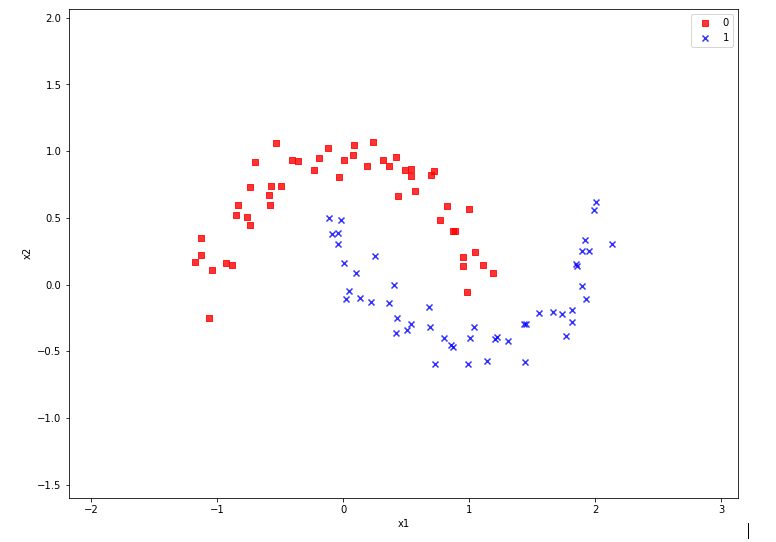
The 2-dim vectors describing the data points are associated with target values of “0” and “1” – with “0” describing the membership in the upper cluster and “1” the membership in the lower cluster of points. We see at once that any hyperplane – in this case a one dimensional, but curved line – separating the data clusters requires some non-linear description with respect to x1 and x2.
We also understand that we need some special plotting technique to visualize the separation. Within the named book of Geron we do not find a recipe for such a plot; however you do find example programs on the author’s website for the exercises in the book. Actually, I found some additional hints in a different book “Python Machine Learning” of Sebastian Raschka, pubished by PACKT Publishing, 2016. When I came to Geron’s discussion of the moon dataset I tried to combine it with the plotting approach of Raschka. For me – as a beginner – the whole thing was a very welcome opportunity to do some exercises with a Jupyter notebook and write some small functions for plotting decision regions.
I describe my way of dealing with the moon dataset below – and hope it may help others. However, before we move to Jupyter based experiments I want to give some hints on the SVM approach and Python libraries required.
SVM, “Polynomial Features” and the SVC Kernel
The algorithm behind a SVM performs an analysis of data point vectors in a multidimensional vector space and the distances of the points of different clusters. The strategy to find a separating hyperplane between data point clusters should follow 3 principles:
- We want to guarantee a large separation in terms of metrical distances of outer cluster points to the separation plane.
- We want to minimize the number of of points violating the separation.
- The number of mathematical operations shall be reduced.
If we had some vector analysis a part of our education we may be able to figure out how to determine a hyperplane in cases where a linear separation is sufficient. We adjust the parameters of the linear hyperplane such that for some defined average the distance of carefully chosen cluster points to the plane is maximized. We could also say that we try to “maximize” the margins of the data clusters to the hyperplane (see the book of Raschka, cahpter 3, around page 70). We can moderate the “maximize” strategy by some parameters allowing for a narrower margin not to get too many wrongly placed data points. Thus we would avoid overfitting. But what to do about a non-linear separation surface?
Non-linearity can be included by a trick: Polynomial variations of the data variables – i.e. powers of the data variables – are added as new so called slack variables to the original data sets – thereby extending the dimensionality of the sets. In the extended new vector space data which previously were not separable can appear in clearly separated regions.
A SciKit-Learn Python class “PolynomialFeatures” supports variations in the combination of powers of the original data up to a limiting total power (e.g. 3). If the 2 dim data variables are x1 and x2, we may e.g. include x1**3, x2**3, x2*x1**2, x1*x2**2 and x1*x2 as new variables. On the extended vector space we could then apply a conventional linear analysis again.
Such a linear analysis is provided by a Python module called LinearSVC which is part of “sklearn.svm”, which provides SVM
related classes and methods. PolynomialFeatures is a class and part of “sklearn.preprocessing”.
Note that higher polynomials obviously will lead to a steep rise in the number of data operations as the dimensionality of the data sets grows significantly due to combinatorics. For many cases it can, however, be shown that it is sufficient to operate with the original data points in the lower dimensional representation space in a special way to cover polynomial extensions or distance calculations for the hyperplane determination in the higher dimensional and extended representation space. A so called “Polynomial Kernel” function takes care of this without really extending the dimensionality of the original datasets.
Note that there are other kernel functions for other types of calculation approaches to determine the separation surface: One approach uses an exponentially weighted distance (Gaussian kernel or RBF-kernel) between points in the sense of a similarity function to add new features (= dimensions) to the representation space. In this case we have to perform mathematical operations on pairs of data points in the original space with lower dimensionality, only.
Thus, different kinds of kernel functions are included in a SciKit-Learn class named “SVC“. All methods work sufficiently well at least for small and medium data sets. For large datasets the polynomial Kernel may scale badly regarding CPU time.
There is another kind of scaling – namely of the data to reasonable value regions. It is well known that data scaling is important when using SVM for the determination of decision surfaces. So, we need another Python class to scale our “moon” data reasonably – “StandardScaler” which is part of sklearn.preprocessing.
Required Python libraries
We assume that we have installed the Python packets sklearn, mathlotlib and numpy in the virtual Python environment for our ML experiments, already. (See previous articles in this blog for the establishment of such an environment on a Linux machine.)
We shall use the option of SciKit-Learn to build pipelines of operations on datasets. So, we need to import the class “Pipeline” from sklearn.pipeline. The “moons dataset” itself is part of the datasets library of “sklearn”.
All in all we will use the following libraries in the forthcoming experiments:
import numpy as np
import matplotlib.pyplot as plt
from matplotlib.colors import ListedColormap

from sklearn.datasets import make_moons

from sklearn.pipeline import Pipeline
from sklearn.preprocessing import StandardScaler
from sklearn.preprocessing import PolynomialFeatures

from sklearn.svm import LinearSVC
from sklearn.svm import SVC
Enough for today.In the next article
The moons dataset and decision surface graphics in a Jupyter environment – II – contourplots
we will acquire some basic tool skills in ML: I shall show how to start a Jupyter notebook and how to create contour-plots. We will need this knowledge later on for doing experiments with our moons data set and to visualize the results of SVM algorithms for classification.