Last week I stared preparing posts for my new blog on Machine Learning topics (see the blog-roll). During my studies last week I came across a scientific publication which covers an interesting topic for ML enthusiasts, namely the question what kind of statistical distributions we may have to deal with when working with data of natural objects and their properties.
The reference is:
S. A. FRANK, 2009, “The common patterns of nature”, Journal of Evolutionary Biology, Wiley Online Library Link to published article
I strongly recommend to read this publication.
It explains statistical large-scale patterns in nature as limiting distributions. Limiting distributions result from an aggregation of the results of numerous small scale processes (neutral processes) which fulfill constraints on the preservation of certain pieces of information. Such processes will damp out other fluctuations during sampling. The general mathematical approach to limiting distributions is based on entropy maximization under constraints. Constraints are mathematically included via Lagrangian multipliers. Both are relatively familiar concepts. The author explains which patterns result from which basic neutral processes.
However, the article also discusses an intimate relation between aggregation and convolutions. The author furthermore presents an related interesting analysis based on Fourier components and respective damping. For me this part was eye-opening.
The central limit theorem is explained for cases where a finite variance is preserved as the main information. But the author shows that Gaussian patterns are not the only patterns we may directly or indirectly find in the data of natural objects. To get a solid basis from a spectral point of view he extends his Fourier analysis to the occurrence of infinite variances and consequences for other spectral moments. Besides explaining (truncated) power law distributions he discusses aspects of extreme value distributions.
All in all the article provides very clear ideas and solid arguments why certain statistical patterns govern common distributions of natural objects’ properties. As ML people we should be aware of such distributions and their mathematical properties.
we have studied the transformation of an ellipse by a shear operation. The coordinates of points on an ellipse and the components of respective position vectors fulfill a quadratic equation (quadratic form):
The superscript “T” symbolizes the transposition operation. The symmetric (2×2)-matrix \( \pmb{\operatorname{A}}_q^O \) defines the original, unsheared ellipse. The suffix “q” indicates the quadratic form. I have shown how the shear parameter λS impacts the coefficients of a corresponding (2×2)-matrix \(\pmb{\operatorname{A}}_q^S \) that defines the sheared ellipse.
What I have not done in the last post is to show how our matrix \(\pmb{\operatorname{A}}_q^S \) is related to a shear matrix \(\pmb{\operatorname{M}}_{sh} \) (see the first post), which describes the effect of the shear on the vectors \( \left(\,x_o,\, y_o\,\right)^T \). I am going to discuss this below. The given matrix relations will also be valid for general n-dimensional ellipsoids.
Matrix relations as discussed below are helpful to accelerate numerical calculations as Numpy (in cooperation with libraries for your OS) provides highly optimized modules for matrix operations. n-dimensional ellipsoids furthermore characterize hyper-surfaces of multivariate normal distributions which appear in certain areas of Machine Learning and respective data.
Matrix describing a centered n-dimensional ellipsoid
We consider n-dimensional and centered ellipsoids whose symmetry centers coincide with the origin of the Euclidean coordinate system [ECS] we work with. A position vector \(\left(\,x_1^o,\, x_2^o\, \cdots x_n^o \right)^T \)
is a vector drawn from the origin to a point on the ellipsoid’s hyper-surface. Note that a general vector of a vector space has no reference to a coordinate system’s origin. Therefore the distinction. A general ellipsoid is defined by a quadratic form in the components of its position vectors. The quadratic form is equivalent to the following matrix equation
where \(\pmb{\operatorname{A}}_{qn}^O \) now represents a symmetric (nxn)-matrix. The “\( \circ \)” symbolizes a matrix product.
Note: A coefficient \( \delta \gt 0 \) which we have used in previous posts on the right side of the equation can be included in the coefficient values of the matrix).
Note that the equations above define an ellipsoid up to a translation vector. This is reflected in the fact that the above equation does not create any linear terms.
Quadratic forms not only define ellipsoids. For an ellipsoid we have to assume that the determinant of\(\pmb{\operatorname{A}}_{qn}^O \) is > 0 and that the matrix is invertible:
Note that you could choose an ECS in which the ellipsoid’s principal axes would align with the ECS’s coordinate axes. Such a choice would correspond to a PCA-transformation of the vector data. \(\pmb{\operatorname{A}}_{qn}^O \) would then become diagonal. This corresponds to the fact that a symmetric matrix always has an eigenvalue-decomposition.
Equation of the quadratic form for the sheared ellipsoid
In the first post of this series I have defined a (invertible) shear matrix as a unipotent matrix \( \pmb{\operatorname{M}}_{sh} \) with all coefficients of the lower triangular part, off the diagonal, being equal to 0.0 and all elements on the diagonal being equal to 1:
So an inverse matrix \( \pmb{\operatorname{M}}_{sh}^{-1} \) exists. Shearing our original ellipse (with position vectors \( \pmb{x_o} \)) leads to new vectors \( \pmb{x_S} \):
Σ is a diagonal (nxm)-matrix with singular values. The column-vectors of U and V are orthogonal singular vectors. Geometrically, U and V can be interpreted s rotational operations.
Therefore, we can decompose a (nxn) upper triangular shear-matrix into two orthonormal (nxn)-matrices U and V plus a diagonal matrix Σ :
This gives us an alternative form to define the inverse shear matrix. Note that the order of the matrices in the matrix products is essential.
An example for the case of a sheared ellipse
We use the example of a sheared ellipse discussed in the last post to verify the results above numerically for a 2-dim case. To write a respective Python/Numpy-program is simple. I will just give you my numerical results below.
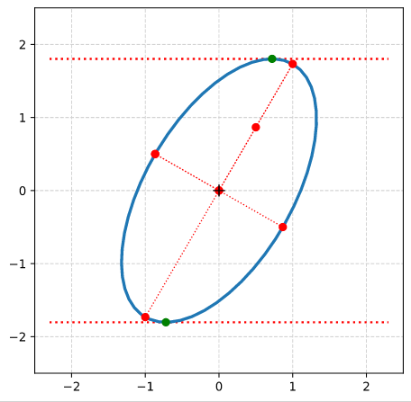
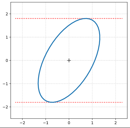
We have used an ellipse with the longer and shorter primary axes having values a = 2 and b = 1, respectively. The ellipse was rotated by 60° against the ECS-axes.
The respective (2×2)-matrix \( \pmb{\operatorname{A}}_q^O \) had the following coefficients
We have shown how a shear matrix \( \pmb{\operatorname{M}}_{sh} \) transforms the matrix \(\pmb{\operatorname{A}}_{qn}^O \) which defines an un-sheared n-dimensional ellipsoid into a matrix \(\pmb{\operatorname{A}}_{qn}^S \) defining its sheared counterpart. We have also had a glimpse on a SVD decomposition of a shear matrix. The results will enable us in the next post to apply shear operations on a concrete example of a 3-dimensional ellipsoid.
Post III focused on the shearing of a circle, which was centered in the Euclidean coordinate system [ECS] we worked with. The shear operation resulted in an ellipse with an inclination against the coordinate axes of our ECS. This was interesting regarding four points:
A circle, which is centered in a chosen ECS, exhibits a continuous rotational symmetry (isotropy). This obviously allows for a decomposition of a shear operation into a sequence of two affine operations in the chosen ECS: a scaling operation (with different factors along the coordinate axes) followed by a rotation (or the other way round). Equivalently: We could switch to another specific ECS which is already rotated by a proper angle against our originally chosen ECS and just perform a scaling operation there. The rotation angle is determined by the shear parameter λ. This seems to stand in some contrast to the shearing of figures with only discrete rotational symmetries: We saw for rectangles and cubes that an additional rotation was required to replace the shear operation by a sequence of scaling and rotation operations.
Points (x, y) of circles and ellipses are described by quadratic forms in two dimensions (with some real coefficients α, β, γ, δ):
\[
\alpha \,x^2 \, + \, \beta \, x \, y \, + \, \gamma \, y^2 \:=\: \delta
\]
Quadratic forms play a general role in the mathematical description of cone-sections. (Ellipses are the results of specific cone-sections.)
Ellipses also result from projections of multi-dimensional ellipsoids onto two-dimensional coordinate planes. Multi-dimensional ellipsoids are described by quadratic forms in an ECS covering the ℝn.
Hyper-surfaces for constant probability density values of multivariate normal vector distributions form multi-dimensional ellipsoids. Here we have a link to Machine Learning where key properties of certain objects are often ruled by Gaussian distributions.
From the first point we may expect that a shear operation applied to a multi-dimensional sphere will result in a multi-dimensional ellipsoid – and that such an operation could be replaced by scaling the original sphere (with different factors along n coordinate axes of a n-dimensional ECS) followed by a rotation (or vice versa). We will explicitly investigate this for a 3-dimensional sphere in the next post.
If our assumption were true we would get a first glimpse of the fact that a general multivariate standard distribution can be created by applying a sequence of distinct affine (i.e. linear) operations to a spherical probability distribution. This is discussed in detail in another post-series in this blog.
What is a bit confusing at the moment is that a replacement of a shear operation by simpler affine operations in general seems to require at least two rotations, but only one when we work with centered isotropic bodies. We come back to this point when we discuss the decomposition of a shear matrix by the so called SVD-procedure.
In the previous post of this series we have used the radius of the circle and the shearing parameter λ to derive analytical expressions for the coordinates of special points with extremal values on our ellipse
Points with maximal and minimal y-coordinate values.
Points with a maximal or minimal distance to the symmetry center of the ellipse. I.e. the end-points of the principal diameters of the ellipse.
From the fact that shearing does not change extremal values along the axis perpendicular to the sharing direction we could easily determine the lengths of the ellipse’s principal axes and the inclination angle of the longer axis with the x-axis of our Euclidean coordinate system [ECS].
What do we have in addition? In another mini-series on ellipses
I have meanwhile described how the geometry of an ellipse is related to its quadratic form and respective coefficients of a symmetric matrix. I call this matrix Aq. It forces the components of position vectors to fulfill an equation based on a quadratic polynomial. Furthermore Aq‘s eigenvalues and eigenvectors define the lengths of the ellipse’s principal axes and their inclination to the axes of our chosen ECS. The matrix coefficients in addition allow us to determine the coordinates of the points with extremal y-values on an ellipse. We will use these results later in the present post.
Objectives of this post: Shearing of a centered, rotated ellipse
In this post I want to show that shearing a given centered, but rotated original ellipse EO results in another ellipse ES with a different inclination angle and different sizes of the principal axes.
In addition we will derive the relations of the shearing parameter λS with the coefficients of the symmetric matrix \(\pmb{\operatorname{A}}_q^S \) that defines ES. I also provide formulas for the dependence of ES‘s geometrical properties on the shear parameter λS.
There are two basic prerequisites:
We must show that the application of a shear transformation to the variables of the quadratic form which describes an ellipse EO results in another proper quadratic form and a related matrix \(\pmb{\operatorname{A}}_q^S \).
The coefficients of the resulting quadratic form and of \(\pmb{\operatorname{A}}_q^S \) must fulfill a mathematical criterion for an ellipse.
We expect point 1 to be valid because a shear operation is just a linear operation.
To get some exercise we approach our goals by first looking at the simple case of shearing an axis-parallel ellipse before extending our considerations to general ellipses with an inclination angle against the coordinate axes of our chosen ECS.
This post requires Javascript to display formulas!
A centered, rotated ellipse can be defined by matrices which operate on position-vectors for points on the ellipse. The topic of this post series is the relation of the coefficients of such matrices to some basic geometrical properties of an ellipse. In the previous posts
we have found that we can use (at least) two matrix based approaches:
One reflects a combination of two affine operations applied to a unit circle. This approach led us to a non-symmetric matrix, which we called AE. Its coefficients ((a, b), (c, d)) depend on the lengths of the ellipses’ principal axes and trigonometric functions of its rotation angle.
The second approach is based on coefficients of a quadratic form which describes an ellipse as a special type of a conic section. We got a symmetric matrix, which we called Aq.
We have shown how the coefficients α, β, γ of Aq can be expressed in terms of the coefficients of AE. Another major result was that the eigenvalues and eigenvectors of Aq completely control the ellipse’s properties.
Furthermore, we have derived equations for the lengths σ1, σ2 of the ellipse’s principal axes and the rotation angle by which the major axis is rotated against the x-axis of the Cartesian coordinate system [CCS] we work with.
We have also found equations for the components of the position vectors to those points of the ellipse with maximum y-values.
In this post we determine the components of the vectors to the end-points of the ellipse’s principal axes in terms of the coefficients of Aq. Afterward we shall test our formulas by a Python program and plots for a specific example.
Reduced matrix equation for an ellipse
Our centered, but rotated ellipse is defined by a quadratic form, i.e. by a polynomial equation with quadratic terms in the components xe and ye of position vectors to points on the ellipse:
The quadratic polynomial can be formulated as a matrix operation applied to position vectors vE = (xE, yE)T. With the the quadratic and symmetric matrix Aq
Method 1 to determine the vectors to the principal axes’ end points
My readers have certainly noticed that we have already gathered all required information to solve our task. In the first post of this series we have performed an eigendecomposition of our symmetric matrix Aq. We found that the two eigenvectors of Aq for respective eigenvalues λ1 and λ2 point along the principal axes of our rotated ellipse:
This is trivial regarding the algebraic operations, but results in lengthy (and boring) expressions in terms of the matrix coefficients. So, I skip to write down all the terms. (We do not need it for setting up ordered numerical programs.)
Remember that you could in addition replace (α, β, γ) by coefficients (a, b, c, d) of matrix AE. See the first post of this series for the formulas. This would, however, produce even longer equation terms.
We pick the yE with the positive term in the following steps. (The way for the solution with the negative term in yE is analogous.) The square of yE is:
A detailed analysis also for the other yE-expression (see above) leads to further solutions for the coordinates (=vector component values) of points with extremal values for the radii. These are the end-points of the principal axes of the ellipse:
I leave it to the reader to expand the convenience variables into terms containing the original coefficients α, β, γ.
Plots
It is easy to write a Python program, which calculates and plots the data of an ellipse and the special points with extremal values of the radii and extremal values of ye. The general steps which I followed were:
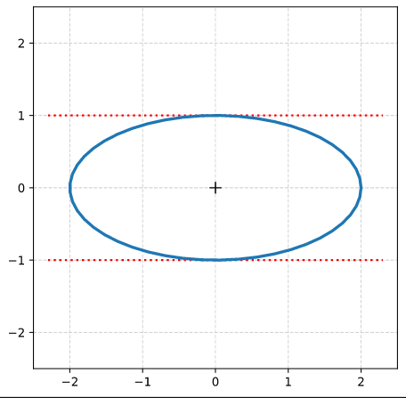
Step 0: Create 100 points a unit circle. Save the coordinates in Python lists (or Numpy arrays). Use Matplotlib’s plot(x,y)-function to plot the vectors.
Step 1: Create an axis-parallel ellipse with values for the axes ha = 2.0 and hb = 1.0 along the x- and the y-axis of the Cartesian coordinate system [CCS]. Do this by applying a diagonal scaling matrix Dσ1, σ2 (see the first post of this series).
Step 2: Rotate the ellipse bei π/3 (60 °). Do this by applying a rotation matrix Rπ/3 to the position vectors of your ellipse (with the help of Numpy). Alternatively, you can first create the matrices, perform a matrix multiplication and then apply the resulting matrix to the position vectors of your unit circle.
(The limiting lines have been calculated by the formulas given above.)
Step 3: Determine the coefficients of combined matrix AE = Rπ/3 ○ Dσ1, σ2
I got for the coefficients ( (a, b), (c, d) ) of AE :
A_ell =
[[ 1.         -0.8660254 ]
[ 1.73205081  0.5       ]]
Step 3: Determine the coefficients of the matrix Aq by the formulas given in the first post of this series. I got
A_q =
[[ 3.25       -1.29903811]
[-1.29903811  1.75      ]]
For δ I got:
delta = 4.0
which is consistent with the length-values of the principal axes.
Step 4: Determine values for the eigenvalues λ1 and λ2 from the Aq-coefficients by the formulas given in the first post. Also calculate them by using Numpy’s
eigenvalues, eigenvectors = numpy.linalg.eig(A_q). Theory tells us that these values should be exactly λ1 = 4 and λ1 = 1. I got
Eigenvalues from A_q: lambda_1 = 4. :: lambda_2 = 1.
Step 5: Determine the components of the normalized eigenvectors with the help of numpy.linalg.eig(A_q). I got:
Components of normalized eigenvectors by theoretical formulas from A_q coefficients:
ev_1_n :  -0.8660254037844386  :  0.5000000000000002
ev_2_n :  0.5000000000000001  :  0.8660254037844385

Eigenvectors from A_q via numpyy.linalg.eig():
ev_1_num :  0.8660254037844387  :  -0.5000000000000001
ev_2_num :  0.5000000000000001  :  0.8660254037844387
The deviation between ev_1_n and ev_1_num is just due to a difference by -1. This is correct as the eigenvectors are unique only up to a minus-sign in all components.
Step 6: Calculate the sinus of the rotation angle of our ellipse from Aq– and Aq-coefficients. The theoretical value is sin(2 π/3) = sin(2 pi/3) = 0.8660254037844387. I got:
sin(2. * rotation angle) of major axis of the ellipse against the CCS x-axis from A_E coefficients:
sin_2phi-A_E  =  0.8660254037844388

sin(2. * rotation angle) of major axis of the ellipse against the CCS x-axis from from eigenvectors of A_q:
sin_2phi-ev_A_q =  0.8660254037844387

sin(2. * rotation angle) of major axis of the ellipse against the CCS x-axis from A_q-coefficients:
sin_2phi-coeff-A_q =  0.8660254037844388
Perfect!
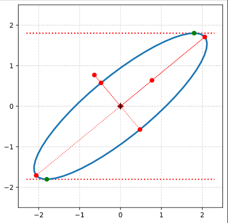
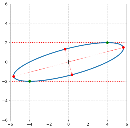
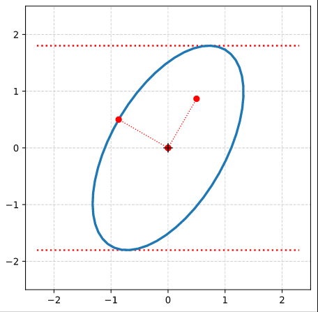
Step 7: Plot the end-points of the normalized eigenvectors of Aq:
Note that in our example case the end-point of the eigenvector along the minor axis must be located exactly on the elliptic curve as the ellipses minor axes has a length of b=1!
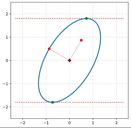
Step 8: Calculate the components of the vectors to data-points of the ellipse with maximal absolute ye-values from the Aq-coefficients given in the previous post. Plot these data-points (here in green color).
Step 9: Calculate the components of the vectors to data-points of the ellipse with maximal values of the radii with the help of the complex formulas presented in this post and plot these points in addition.
Conclusion
In this mini-series of posts we have performed some small mathematical exercises with respect to centered and rotated ellipses. We have calculated basic geometrical properties of such ellipses from the coefficients of matrices which define ellipses in algebraic form. Linear Algebra helped us to understand that the eigenvectors and eigenvalues of a symmetric matrix, whose coefficients stem from a quadratic equation (for a conic section), control both the orientation and the lengths of the ellipse’s axes completely.
This knowledge is useful in some Machine Learning [ML] context where elliptic data appear as projections of multivariate normal distributions. Multivariate Gaussian probability functions control properties of a lot of natural objects. Experience shows that certain types of neural networks may transform such data into multivariate normal distributions in latent spaces. An evaluation of the numerical data coming from such ML-experiments often delivers the coefficients of defining matrices for ellipses.
In my blog I now return to the study of with shearing operations applied to circles, spheres, ellipses and 3-dimensional ellipsoids. Later I will continue with the study of multivariate normal distributions in latent spaces of Autoencoders. For both of these topics the knowledge we have gathered regarding the matrices behind ellipses will help us a lot.
I have discussed how the coefficients of two matrices which can be used to define a centered, rotated ellipse can be used to calculate geometrical properties of the ellipse:
The lengths σ1, σ2 of the ellipse’s principal axes and the rotation angle by which the major axis is rotated against the x-axis of the Cartesian coordinate system [CCS] we work with.
But there are other properties which are interesting, too. A centered, rotated ellipse has two points with extremal values in their y-coordinates. Can we express the coordinates – or equivalently the components of respective position vectors – in terms of the basic matrix coefficients?
The answer is, of course, yes. This post provides a derivation of respective formulas.
Matrix equation for an ellipse
In the last post we have shown that a centered ellipse is defined by a quadratic form, i.e. by a polynomial equation with quadratic terms in the components xE and yE of position vectors for points of the ellipse:
The quadratic polynomial can be formulated as a matrix operation applied to position vectors vE of points on an ellipse. With the the quadratic and symmetric matrix Aq
We now follow the alternative solution for yE (see above). After a calculation of the yE-values from the derived xE values, we get the components for the two position vectors to the points with extremal y-values on the ellipse:
Solution in terms of the coefficients of an alternative matrix AE
In my previous post I have discussed yet another matrix AE which also can be used to define an ellipse. This matrix summarizes two affine transformations of a centered unit circle: AE = Rφ ○ Dσ1, σ2. Dσ1, σ2.
You find the relations between the coefficients (a, b, c, d) of matrix AE and the coefficients (α, β, γ) of matrix Aq in my previous post. This will allow you to calculate the vectors to the extremal points of an ellipse in terms of the coefficients (a, b, c, d).
Conclusion
In this post we have again used the coefficients of a matrix which defines an ellipse via a quadratic form to get information about a geometrical property.
We can now calculate the components of the position vectors to the two points of an ellipse with extremal y-values as functions of the matrix coefficients.
I will show you how to calculate the components of the end points of the principal axes of the ellipse with the help of our matrix for a quadratic form. I will also use our theoretical results for plots of some ellipses’ axes and of their extremal points. We will also compare theoretical predictions with numerically evaluated values.