Blender – even on old laptops a graphics card increases rendering performance

My present experiments with Blender on my old laptop take considerable time to render- especially animations. So, I got interested in whether rendering on the laptop’s old Nvidia card, a GT 645M, would make a difference in comparison to rendering on the available 8 hyperthreaded cores of the CPU. The laptop’s CPU is an old one, too, namely an i7-3632QM. The laptop’s operative system is Opensuse Leap 15.3. The system uses Optimus technology. To switch between the Nvidia card and the Intel graphics I invoke Suse’s Prime Select application on KDE.

I got a factor of 2 up to 5.2 faster rendering on the GPU in comparison to the CPU. The difference depends on multiple factors. The number of CPU cores used is an important one.

How to activate GPU rendering in Blender?

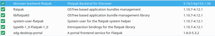
Basically three things are required: (1) A working recent Nvidia driver (with compute components) for your graphics card. (2) A certain setting in Blender’s preferences. (3) A setting for the Cycles renderer.

Regarding the CUDA toolkit I quote from Blender’s documentation

Normally users do not need to install the CUDA toolkit as Blender comes with precompiled kernels.

With respect to required Blender settings one has to choose a CUDA capable device via the menu point “Preferences >> System”:

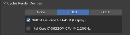
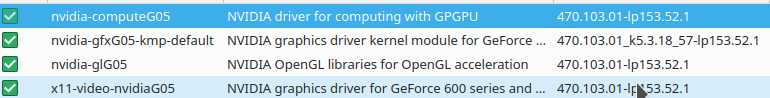
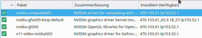
You may also select both the GPU and the CPU. Then rendering will be done both on the GPU and the CPU. My graphics card unfortunately only understands a low level of CUDA instructions. The Nvidia driver I used is of version 470.103.01, installed via Opensuse’s Nvidia community repository:

In addition, you must set an option for the Cycles renderer:

With all these settings I got a factor of 2 up to > 6 faster rendering on the GPU in comparison to a CPU with multiple cores.

The difference in performance, of course, depends on

  • the number of threads used on the CPU with 8 (hyperthreaded) cores available to the Linux OS
  • tiling – more precisely the “tile size” – in case of the GPU and the CPU

All other render options with the exception of “Fast G” were kept constant during the experiments.

Scene Setup

To give the Blender’s Cylces renderer something to do I set up a scene with the following elements:

  • a mountain-like landscape (via the A.N.T Landscape Add-On) with a sub-dividion of 256 to 128 – plus subdivision modifier (Catmull-Clark, render level 2, limit surface quality 3) – plus simple procedural texture with some noise and bumps
  • a plane with an “ocean” modifier (no repetition, waves + noisy bump texture for the normal to simulate waves)
  • a world with a sky texture of the Nishita type ( blue sky by much oxygen, some dust and a sun just above the horizon)

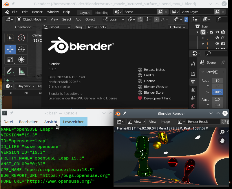
The scene looked like

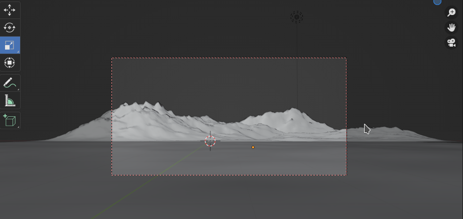
The central red rectangle marks the camera perspective and the area to be rendered. With 80 samples and a resolution of 1200×600 we get:

The hardest part for the renderer is the reflection on the water (Ocean with wave and texture). Also the “landscape” requires some time. The Nishita world (i.e. the sky with the sun), however, is rendered pretty fast.

Required time for rendering on multiple CPU cores

I used 40 samples to render – no denoising, progressive multi-jitter, 0 minimum bounces.
Other settings can be found here:


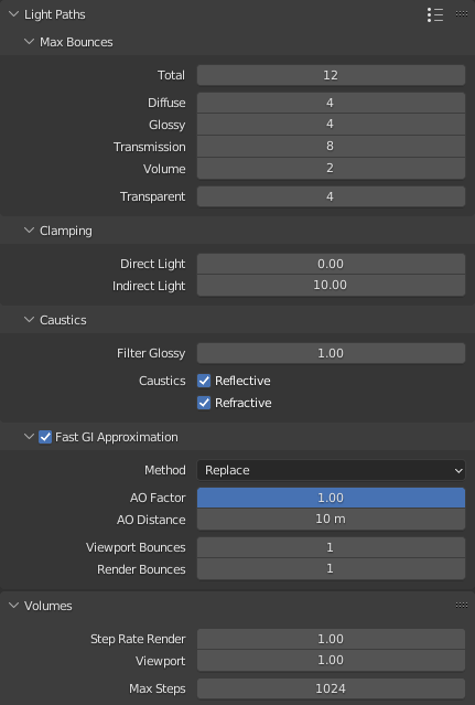
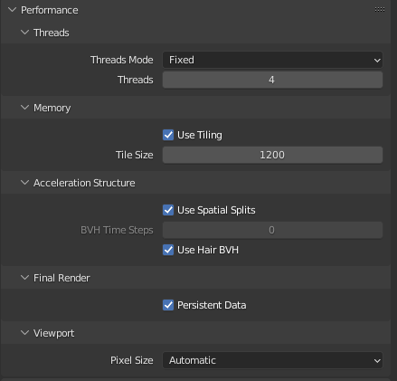
The number of threads, the tile size and the use of the Fast CI approximation were varied.
The resolution was chosen to be 1200×600 px.

All data below were measured on a flatpak installation of Blender 3.1.2 on Opensuse Leap 15.3.

tile size threads Fast GI time
64 2 no 82.24
128 2 no 81.13
256 2 no 81.01
32 4 no 45.63
64 4 no 43.73
128 4 no 43.47
256 4 no 43.21
512 4 no 44.06
128 8 no 31.25
256 8 no 31.04
256 8 yes 26.52
512 8 no 31.22

A tile size of 256×256 seems to provide an optimum regarding rendering performance. In my experience this depends heavily on the scene and the chosen image resolution.

“Fast GI” gives you a slight, but noticeable improvement. The differences in the rendered picture could only be seen in relatively tiny details of my special test case. It may be different for other scenes and illumination.

Note: With 8 CPU cores activated my laptop was stressed regarding CPU temperature: It went up to 81° Celsius.

Required time for rendering on the mobile GPU

Below are the time consumption data for rendering on the mobile Nvidia GPU 645M:

tile size Fast GI time
64 no 18.3
128 no 16.47
256 no 15.56
512 no 15.41
1024 no 15.39
1200 no 15.21
1200 yes 12.80

Bigger tile sizes improve the GPU rendering performance! This may be different for rendering on a CPU, especially for small scenes. There you have to find an optimum for the tile size. Again, we see an effect of Fast GI.

Note: The temperature of the mobile graphics card never rose above 58° Celsius. I measured this whilst rendering a much bigger image of 4800×2400 px. I therefore think that the temperature stress Blender rendering exerts on the GPU is relatively smaller in comparison to the heat stress on a CPU.

Required time for rendering both on the CUDA capable mobile GPU and the CPU

As the CPU is CUDA capable one can activate CUDA based rendering on the CPU in addition to the GPU in the “preferences” settings. With 4 CPU cores this brings you down to around 11 secs, with 8 cores down to 10 secs.

tile size threads Fast GI time
64 4 no 11.01
128 8 no 10.08

Conclusion

Even on an old laptop with Optimus technology it is worthwhile to use a CUDA capable Nvidia graphics card for Cycles based rendering in Blender experiments. The rise in temperature was relatively low in my case. The gain in performance may range from a factor 2 to 5 depending on how many CPU cores you can invoke without overheating your laptop.

Ceterum censeo: The worst living fascist and war criminal today, who must be isolated, denazified and imprisoned, is the Putler.


Blender – complexity inside spherical and concave cylindrical mirrors – VI – first experiment with a half-sphere

I had some fun yesterday with a first experiment I did in Blender with a fully reflective concave half-sphere. This is a further step in this series about the construction of some special reflecting surfaces in Blender for virtual optical experiments.

Blender – complexity inside spherical and concave cylindrical mirrors – I – some impressions
Blender – complexity inside spherical and concave cylindrical mirrors – II – a step towards the S-curve
Blender – complexity inside spherical and concave cylindrical mirrors – III – a second step towards the S-curve
Blender – complexity inside spherical and concave cylindrical mirrors – IV – reflective images of a Blender variant of Mr Kapoor’s S-curve
Blender – complexity inside spherical and concave cylindrical mirrors – V – a video of S-curve reflections

One of the most spectacular effect in a NASA movie about a real half-sphere (see the first post of this series) is the virtual finger that seems to come out of the sphere when the physicist moved his own finger towards the center. I thought this might be a nice Blender experiment on a free day with bad weather outside. The finger had to be replaced by a small lengthy NURBS based cylinder in Blender. The main objective was to find some cylinder-like figure coming out of a half-sphere built in Blender. But as I was playing around I shot some additional images of the half-sphere from different positions to verify the appearance of ring-like patterns at the outer edges of the half-sphere, too.

Building the half-sphere

I created the half-sphere for this experiment as a mesh with 64×64 faces, which I cut into two parts afterwards. I added the “subdivision modifier” at the end to get a smooth surface. But, probably, you could also have started with a high resolution Nurb sphere. I have not yet tested which methods results in faster rendering. Reflectivity was achieved by setting the material to be fully metallic without any roughness. The base color of the material was set to pure white.

Scene setting

The geometrical setup I choose for this post is the following:

The image above reflects my first camera perspective. What we want to see from this perspective is a mirrored pattern of the cylinder-like (Nurbs) object – appearing in front of the background mirror-surface and opposite of the real object. Such an appearance would of course just be an illusion, but is the result of simple optics. The light rays reaching the camera stem of course from the inner surface of the half sphere. Note that the cylinder is placed on the central symmetry axis of the half-sphere. We later give it a metallic red surface. Note also that the Nurb’s cylinder is an open figure at both ends and not a solid one. So, we will get some tiny reflection patterns on the inside of the cylinders, too.

The small sphere is placed off the symmetry axis to show a different reflection effect. I gave it a green color. A few light sources have been placed at various positions.

As a background I chose again a kind of dusk with a “sun” just above the horizon. This gives us a distinct contrast rich orange-yellow horizontal stripe, which will later help us to identify multiple reflections inside the half-sphere. Remember that we should get an inner part of the half-sphere showing a sharp ring-like edge marking the border-line where the first double reflection occurs. Other ring-like shapes, which a camera positioned on the central symmetry axis and looking towards the half-sphere’s center should “see”, appear in the outer areas of the half-sphere. The distance between these ring like structures should systematically become smaller.

At the bottom of the half-sphere I have also added an extended reflective plane. This helps us later to watch different reflection patterns coming from two different angles towards the camera. The half sphere is placed a bit above the ground level, i.e. above the plane. This leads to incomplete rings resulting from multiple reflections of the horizon line.

Result for a camera position above and sideways of the cylinder close to the half-sphere

From the perspective shown above we get the following rendered image:

So, indeed we see an artificial cylindrical “figure” coming out of the inner part of the half sphere opposite the real red cylinder. In addition, the sharply edged inner area of the half-sphere is clearly visible – here a bit distorted as our camera is placed off the central axis. At the top of the half-sphere the effects of multiple reflections stemming from the horizontal line can clearly be seen. The green sphere leads to a reflection pattern which already appeared at the concave side of the S-curve (see the previous posts).

Changed camera perspective high above the central symmetry axis

In a second experiment I placed the camera above the central axis at quite a distance away from the half-sphere and relatively high in z-direction. A yellow and somewhat extended light source has been added to get one more reflection pattern.

We clearly see the expected ring like structures due to multiple reflections at the upper edge of the half sphere. It seems that the basic optics works well in Blender. Something which is unrealistic in the images I create is the lossless reflection; in reality reflective patterns would get a bit weaker in intensity with every reflection.

Camera perspective from a position on the central symmetry axis

If we put the camera down to the central axis, the green sphere to the same height and switch off the yellow light sources we get the following result:

A bit off the symmetry axis

Let us eventually get the camera a bit offside the symmetry axis and move the green sphere into a position closer to, but not onto the main axis. Then we get the following picture:

Conclusion

As we expected after our experience with the S-curve we get interesting reflection patterns from a mirroring half-sphere. We showed that Blender reproduces a pattern where a figure seems to grow out of the half-sphere when we move an elongated body into the sphere along the main symmetry axis. We also saw a strong dependency of the reflection patterns on the position of the camera. So, all is well prepared for more experiments.
And, again, a basic lesson is: Some things appear bigger than they are, because we look at a bloated image instead of the real thing. If only things were that easy in politics, too.

Ceterum censeo: The worst living fascist and war criminal today, who must be isolated, denazified and imprisoned, is the Putler.


Blender – complexity inside spherical and concave cylindrical mirrors – V – a video of S-curve reflections

After some months without much Blender activities I now have some days to continue with the experiments in this series.

Blender – complexity inside spherical and concave cylindrical mirrors – I – some impressions
Blender – complexity inside spherical and concave cylindrical mirrors – II – a step towards the S-curve
Blender – complexity inside spherical and concave cylindrical mirrors – III – a second step towards the S-curve
Blender – complexity inside spherical and concave cylindrical mirrors – IV – reflective images of a Blender variant of Mr Kapoor’s S-curve

To get a fresh start I thought it might be funny to get a more dynamic view on the S-curve. I am going to make movies especially for the effects created by a half-sphere later on as we expect some spatial effects there. Look at the NASA movie I referred to in my first post of this series.

The images published in my last posts show that the concave part of the S-curve is the interesting one regarding reflections. The Gaussian curvature is positive there at every point. Therefore we get multiple reflections and large scale reshaping of simple regular figures or bodies. It gives us a first idea about what a half-sphere may create by the reflection of light rays.

A movie

Below I put the video with somewhat reduced resolution but the download of the 1.5 MB may still take some time. An additional link allows you to download an mp4-file with a resolution of 1000×500 px.

Link to movie with a bit higher resolution.
mv_SC_1000_mp40001-0200.mp4

Some remarks

All reflection patterns stem from 3 fully reflective, metallic spheres which are moved in front of the S-curves surface.
The “organic” jelly-like appearance of the pattern dynamics is partially due to the spherical form of the figures. Spherical surfaces lead to soft edges of the reflective patterns. The fully reflective surface of the spheres helps in addition.
The enlargements of some patterns during their object’s movement are due to the curvature of the S-curve in both direction, but especially along the longer symmetry axis, i.e. in the direction of the camera. This curvature increases the area from where light rays emitted from the surface of the spheres can hit the camera.
The separation and merging of some parts of the reflection patterns is due to single reflections of the spheres on fitting upper and lower parts of the S-curve. Such reflective patterns can also merge with reflective patterns emerging from central parts of the S-curve.
Multiple up/down-reflections can be seen in the beginning for the green sphere and at the end of the movie for the red sphere.

Conclusion

Moving objects in front of the S-curve make this surface even more interesting. Again all tribute to Mr Kapoor whose S-curve object at the Kistefoss museet gave me the idea to reconstruct something similar in Blender.
Stay tuned …

Ceterum censeo: The worst living fascist and war criminal today, who must be isolated, denazified and imprisoned, is the Putler.


Replacing unstable Blender 2.82 on Leap 15.3 with flatpak or snap based Blender 3.1

I wanted to work a bit more with my S-curve project in Blender. See e.g.

Blender – complexity inside spherical and concave cylindrical mirrors – IV – reflective images of a Blender variant of Mr Kapoor’s S-curve

At my present location I have to use my old but beloved laptop. As a new start in the project I just wanted to make a little movie showing dynamic changes in the reflections of some moving spheres in front of the S-curve’s metallic surface. As I had already created a few Blender movies some years ago I expected this to be an easy job. But I ran into severe trouble. A major reason was the fact that Opensuse does not provide a reasonably usable RPM of a current Blender versions for Leap 15.3.

I had upgraded the laptop to Leap 15.3 in December, 2022. The laptop has an Optimus system. Of course, I prefer the Nvidia card when creating scenes with Blender. I had had some minor problems with prime-select before. But after recent updates I did not get the Nvidia card running at all – neither with Bumblebee nor with Opensuse’s prime-select. I had to invest an hour to solve this problem. After a complete uninstall of Bumblebee and bbswitch and a de- and re-installation of the Nvidia drivers and suse-prime I got prime-select working in the end.

Just to find that Blender version 2.82 provided by the Leap 15.3 OSS repository was not really stable in a Leap 15.3 environment.

Blender 2.82 unstable on Opensuse Leap 15.3

I tried to create a movie with 100 frames (400×200) in Matroska format with H.264 encoding. Rendering of the complex S-curve reflections with a strongly reduced number of light ray samples still took considerable time with the Cycles renderer on 2 out of 4 real (and 8 hyperthreaded) CPU cores. It happened that the movie – after rendering an hour – was not baked correctly. In some runs Blender crashed after having rendered around 40 frames.

Therefore I changed my policy to rendering just a collection of PNG images. The risk of wasting something like 8 hours of CPU time for a real animation was just too big. But, a new disaster happened when I wanted to open a “video editing”- project in Blender to stitch the images together to create the final movie. Blender just crashed. Actually, Blender crashed on Leap 15.3 whenever I tried to open any project type other than “General”. Not funny … I had not experienced something like this on Leap 15.2.

Unfortunately, and in contrast to Tumbleweed there is no official and recent version of Blender available for Leap 15.3. So much about stability and reliability of Leap. What to do?

Canonical’s snap service or Flatpak to the rescue

I had read about SNAP of Canonical before – but never tried it. Canonical’s strange side steps during the evolution of Linux have always been disturbing for me. Regarding “snap” I also had a newspaper article in mind about a controversy with Linux Mint – with claims that snap has closed proprietary components and is transmitting telemetry data to Canonical. Working with root rights …

Therefore, a flatpack installation had to be considered, too…. Risks are small on my old laptop. I just tried – despite concerns and doubts regarding snap.

Blender 3.1 via “snap

I just followed the instructions for Opensuse on https://snapcraft.io/docs/installing-snap-on-opensuse to install “snap” on my Leap 15.3 system. As root:

zypper addrepo --refresh     https://download.opensuse.org/repositories/system:/snappy/openSUSE_Leap_15.3     snappy
zypper install snapd
systemctl enable --now snapd
systemctl enable --now snapd.apparmor
rcsnapd status
# install blender
snap install blender --channel=3.1/stable --classic

Another description can be found here:
https://www.linuxcapable.com/how-to-install-snap-snap-store-snapcraft-on-opensuse-leap-15/

The run-time environment of snap is handled by a daemon “snapd”. We find the majority of the installed files in four directories

/snap           -- 1.1 GB thereof 686 MB for Blender
/usr/lib/snap   -- 48 MB
/var/snap       -- almost nothing 
/var/lib/snapd  -- 360 MB 

In the first directory you also find the installed applications. In my case “Blender 3.1.2”.
The folder “/snap” contains around 1.1 GB. Blender is part of it and consumes 686 MB.

The startup of Blender via

/snap/bin/blender &

takes about 2 secs. Loading my S-curve test file took even longer. Otherwise snap’s Blender version 3.1.2 seemed to work perfectly. All the bugs I had seen with 2.82 were and are gone. And: I could not really notice a difference in performance when working with 3D objects in the Blender viewport. For a render test case I found 17.72 secs per frame on average. Memory release after leaving Blender seemed to be OK.

Blender 3.1 via Flatpak

Then I tried a Blender installation with flatpak. The installation is almost as simple as for snap. See https://www.flatpak.org/ setup/ openSUSE. Which sums up more or less to issuing the following commands :

zypper install flatpak
flatpak remote-add --if-not-exists flathub https://flathub.org/repo/flathub.flatpakrepo
flatpak install flathub org.blender.Blender

The required packages of the Opensuse repository were

Regarding the installation I was surprised to find that flatpak requires much more space than snap. The majority of flatpack files is located in the following folder:

/var/lib/flatpak  -- 2.3 GB, thereof around 628 MByte for Blender

So, in comparison to snap, this makes a remarkable huge difference regarding the required files to provide a working runtime environment! I understand that for just one application many files have to be provided for a stable run-time environment on KDE – but in comparison to the snap installation it appears bloated.

We start flatpak’s Blender via

flatpak run org.blender.Blender &

The startup time was comparable to the snap installation – no difference felt. The test render time per frame was 18.95 secs. So that was 1.2 secs or 6.5 % slower than snap. Reason unclear. The difference after repeated trials was sometimes a bit smaller (4%), but sometimes also bigger (8.5%) -depending on the start order of the blender applications. But on average snap’s Blender was always a bit faster. I regard the difference is not really as problematic. But it is interesting. Memory release worked also perfectly with flatpak’s Blender installation.

Conclusion

Before you start struggling with the Blender 2.82 binary Opensuse provides, it is really worth trying a flatpak-based or a snap-based installation of Blender 3.1.2. On my system both worked perfectly.

Before you make a decision whether to go with flatpak or snap take into account the critical points which were discussed on the Internet regarding proprietary aspects of snap. Personally, I am going to use flatpak for Blender.
Otherwise, my opinion is that distributors like Opensuse should provide an important application as Blender in its present version as a binary and resolve dependencies as soon as possible. For me a flatpack installation is just a compromise. And it cost me a lot of valuable SSD space.

Links

https://www.linux-community.de/ausgaben/ linuxuser/2018/02/dreikampf/
https://hackaday.com/2020/06/24/whats-the-deal-with-snap-packages/
https://www.makeuseof.com/snap-vs-appimage-vs-flatpak/

Ceterum censeo: The worst living fascist and war criminal today who must be isolated, denazified and imprisoned is the Putler.


Switching between Intel and Nvidia graphics cards on an Optimus laptop with Leap 15.3

At my present location an old laptop with an Optimus system still provides me with good services. Recently, I installed Opensuse Leap 15.3 on it. Since then I have tried almost all I can think of to get Bumblebee running smoothly on it. In the end I gave up – sometimes “primusrun” worked, sometimes not – especially with more complex applications like Blender. And even if “primusrun” worked – “optirun” most often did not.

So, I had a look at “prime-select” installed by the packet “suse-prime” of Opensuse. Again I had mixed experiences: This worked sometimes from the command line and sometimes not. There were multiple things which were somehow interwoven:

  • bbswitch intervened or was used by prime-select when switching to Intel – and when it did and turned the nvidia card off, you could activate it again, but afterward the Nvidia device it was not recognized by the native Nvida driver or by prime-select. Most often I had to reboot.<
  • When I was lucky and after reboots got a configuration where the Nvidia driver was loaded in parallel to the i915 for Intel and used “prime-select” together with an init 3 / init 5 sequence the display manager sddm did not come up. Others had this problem, too.
  • To switch between the graphics cards it was absolutely necessary to login into my graphical KDE desktop, use a root terminal and switch to the Nvidia card with prime-select from there. Then I had to log out and if I was lucky the display manager came up and the Nvidia card was really active.

But do not ask me, what I had to do in which order to get the aspired result. All in all the behavior of “prime-select” was a bit unpredictable. Then after updating a lot of packets yesterday I could no longer get prime-select to do the right things any more. Most often I got the message:

ERROR: Unable to query GPU information

Or : No such device found.

Solution Part 1: Deinstallation of unrequired RPMs and reinstallation of required RPMs

In the end I deinstalled Bumblebee (as recommended by posts in Suse forums) and also bbswitch. Afterward I reinstalled the packets “suse-prime” and “plasma5-applet-suse-prime” from the Leap 15.3 Update-repository (i.e. the Update repo for the Enterprise system) and the Nvidia-drivers from Opensuse’s Nvidia repository. I rebooted and my “sddm” display-manager came up – with the Intel driver active – but the Nvidia driver was loaded already nevertheless. Checked with lsmod.

Later, I found that all files in “/etc/prime” had been rewritten. I suspect that I had something in there which was no longer compatible with the latest drivers and prime-versions. In addition the file “90-nvidia.conf” has been replaced in “/etc/X11/xorg.conf.d“.

Solution Part 2: Use the “Suse Prime Selector” applet!

Then I used the applet in the KDE Plasma desktop to switch to Nvidia. This seemed to work and led to no errors. I just had to log out of my KDE Plasma session and in again to work with KDE on a running Nvidia card. (Ignore the message that you have to reboot).
Afterward I also tested switching by using the command “prime-select” as root in a terminal window of the KDE desktop. Worked perfectly, too.

Conclusion

I am not sure what the ultimate reason was to get prime-select running. The deinstallation of Bumblebee and bbswitch? The new Prime and Nvidia configuration files? Or a new udev during other updates?

Anyway – using the Suse Prime Selector applet or just using the command “prime-select” as root in a terminal window inside KDE Plasma has become a very stable way on my Leap 15.3 laptop with KDE to switch between graphics cards reliably. I still have to log in and log out again of the KDE session – but so far I have never experienced any problems with the display-manager again.

Just for information: I am using the following Nvidia drivers packages:

The prime-select packet version is:

Links

https://www.reddit.com/ r/ openSUSE/ comments/ ib9buv/ opensuse_kde_suse_ prime_selector_ applet_for/
https://forums.developer.nvidia.com/ t/ kubuntu-18-04-gives-black-screen-when-sddm-starts-no-login/ 61034/11
https://wiki.archlinux.org/ title/ PRIME# Configure_applications_%20 to_render_using_GPU
https://www.opensuse-forum.de/ thread/ 63871-suse-prime-error-unable-to-query-gpu-information/
https://opensuse.github.io/ openSUSE-docs-revamped-temp/hybrid_graphics/

Ceterum censeo: The worst living fascist and war criminal, who must be isolated, denazified and imprisoned, is the Putler.