
This post requires Javascript to display formulas!
In my previous post of the series
Fun with shear operations and SVD – I – shear matrices and examples created with Blender
Fun with shear operations and SVD – II – Shearing of rectangles and cubes with Python and Matplotlib
Fun with shear operations and SVD – III – Shearing of circles
Fun with shear operations and SVD – IV – Shearing of ellipses
we have studied the transformation of an ellipse by a shear operation. The coordinates of points on an ellipse and the components of respective position vectors fulfill a quadratic equation (quadratic form):
\alpha_o\,x_o^2 \, + \, \beta_o \, x_o y_o \, + \, \gamma_o \, y_o^2 \:=\: \delta_o
\]
An equivalent matrix equation for respective vectors \( \left(\,x_o,\, y_o\,\right)^T \) is
\left(\,x_o,\, y_o\,\right) \,\circ\, \pmb{\operatorname{A}}_q^O \,\circ\, \left(\,x_o,\, y_o\,\right)^T \: = \: \delta_o
\]
The superscript “T” symbolizes the transposition operation. The symmetric (2×2)-matrix \( \pmb{\operatorname{A}}_q^O \) defines the original, unsheared ellipse. The suffix “q” indicates the quadratic form. I have shown how the shear parameter λS impacts the coefficients of a corresponding (2×2)-matrix \(\pmb{\operatorname{A}}_q^S \) that defines the sheared ellipse.
What I have not done in the last post is to show how our matrix \(\pmb{\operatorname{A}}_q^S \) is related to a shear matrix \(\pmb{\operatorname{M}}_{sh} \) (see the first post), which describes the effect of the shear on the vectors \( \left(\,x_o,\, y_o\,\right)^T \). I am going to discuss this below. The given matrix relations will also be valid for general n-dimensional ellipsoids.
Matrix relations as discussed below are helpful to accelerate numerical calculations as Numpy (in cooperation with libraries for your OS) provides highly optimized modules for matrix operations. n-dimensional ellipsoids furthermore characterize hyper-surfaces of multivariate normal distributions which appear in certain areas of Machine Learning and respective data.
Matrix describing a centered n-dimensional ellipsoid
We consider n-dimensional and centered ellipsoids whose symmetry centers coincide with the origin of the Euclidean coordinate system [ECS] we work with. A position vector \(\left(\,x_1^o,\, x_2^o\, \cdots x_n^o \right)^T \)
\pmb{x_o} \: = \: \begin{pmatrix} x_1^o \\ x_2^o \\ \vdots \\ x_n^o \end{pmatrix}
\]
is a vector drawn from the origin to a point on the ellipsoid’s hyper-surface. Note that a general vector of a vector space has no reference to a coordinate system’s origin. Therefore the distinction. A general ellipsoid is defined by a quadratic form in the components of its position vectors. The quadratic form is equivalent to the following matrix equation
\left(\pmb{x_o}\right)^T \,\circ\, \pmb{\operatorname{A}}_{qn}^O \,\circ\, \pmb{x_o} \: = \: 1
\]
where \(\pmb{\operatorname{A}}_{qn}^O \) now represents a symmetric (nxn)-matrix. The “\( \circ \)” symbolizes a matrix product.
Note: A coefficient \( \delta \gt 0 \) which we have used in previous posts on the right side of the equation can be included in the coefficient values of the matrix).
Note that the equations above define an ellipsoid up to a translation vector. This is reflected in the fact that the above equation does not create any linear terms.
Quadratic forms not only define ellipsoids. For an ellipsoid we have to assume that the determinant of\(\pmb{\operatorname{A}}_{qn}^O \) is > 0 and that the matrix is invertible:
\operatorname{det} \left(\pmb{\operatorname{A}}_{qn}^O \right) \: \gt \: 0
\]
Note that you could choose an ECS in which the ellipsoid’s principal axes would align with the ECS’s coordinate axes. Such a choice would correspond to a PCA-transformation of the vector data. \(\pmb{\operatorname{A}}_{qn}^O \) would then become diagonal. This corresponds to the fact that a symmetric matrix always has an eigenvalue-decomposition.
Equation of the quadratic form for the sheared ellipsoid
In the first post of this series I have defined a (invertible) shear matrix as a unipotent matrix \( \pmb{\operatorname{M}}_{sh} \) with all coefficients of the lower triangular part, off the diagonal, being equal to 0.0 and all elements on the diagonal being equal to 1:
\begin{pmatrix}
1 & m_{12} &\cdots & m_{1n}(\ne0) \\
0 & 1 &\cdots & m_{2n} \\
\vdots &\vdots &\ddots &\vdots \\
0 & 0 &\cdots & 1 \end{pmatrix}
\]
Note:
\]
So an inverse matrix \( \pmb{\operatorname{M}}_{sh}^{-1} \) exists. Shearing our original ellipse (with position vectors \( \pmb{x_o} \)) leads to new vectors \( \pmb{x_S} \):
\pmb{x_S} \: =\: \,\pmb{\operatorname{M}}_{sh} \,\circ\, \pmb{x_o}
\]
We insert \( \pmb{x_S} \) into our defining equation of the original ellipsoid to derive a matrix equation for the sheared ellipsoid:
\left[ \, \pmb{\operatorname{M}}_{sh}^{-1} \,\circ\, \pmb{x_S} \, \right]^T \,\circ\, \pmb{\operatorname{A}}_{qn}^O \,\circ\, \left[ \, \pmb{\operatorname{M}}_{sh}^{-1} \,\circ\, \pmb{x_S} \, \right] \: = \: 1
\]
Giving:
\left(\pmb{x_S}\right)^T \,\circ\, \left[ \, \left( \, \pmb{\operatorname{M}}_{sh}^{-1} \, \right)^T \,\circ\, \pmb{\operatorname{A}}_{qn}^O \,\circ\, \, \pmb{\operatorname{M}}_{sh}^{-1} \, \right] \,\circ\, \pmb{x_S} \: = \: 1
\]
This, obviously, is a new definition equation for a quadratic form in the components of \( \pmb{x_S} \) with a matrix
\pmb{\operatorname{A}}_{qn}^S \:=\: \left( \, \pmb{\operatorname{M}}_{sh}^{-1} \, \right)^T \,\circ\, \pmb{\operatorname{A}}_{qn}^O \,\circ\, \, \pmb{\operatorname{M}}_{sh}^{-1}
\]
We also find:
\operatorname{det}\left(\pmb{\operatorname{A}}_{qn}^S \right) \:=\: \operatorname{det}\left(\pmb{\operatorname{A}}_{qn}^O \right) \: \gt \: 0
\]
From this we can conclude with confidence that we again have gotten a n-dimensional ellipsoid.
Inclusion of a SVD eigendecomposition of MS
A “Singular Value Decomposition” [SVD] can be applied to any (nxm)-matrix Q (with n > m):
\pmb{\operatorname{Q}} \:=\: \pmb{\operatorname{U}} \,\circ\, \pmb{\operatorname{\Sigma}} \,\circ\, \, \pmb{\operatorname{V}}^T
\]
The (nxn)-matrix U and the (mxm)-matrix V are orthonormal matrices:
\pmb{\operatorname{U}} \,\circ\, \pmb{\operatorname{U}}^T \:&=\: 1 \\
\pmb{\operatorname{V}} \,\circ\, \pmb{\operatorname{V}}^T \:&=\: 1
\end{align}
\]
Σ is a diagonal (nxm)-matrix with singular values. The column-vectors of U and V are orthogonal singular vectors. Geometrically, U and V can be interpreted s rotational operations.
Therefore, we can decompose a (nxn) upper triangular shear-matrix into two orthonormal (nxn)-matrices U and V plus a diagonal matrix Σ :
\pmb{\operatorname{M}}_{sh} \:=\: \pmb{\operatorname{U}} \,\circ\, \pmb{\operatorname{\Sigma}} \,\circ\, \, \pmb{\operatorname{V}}^T
\]
This leads to
\pmb{\operatorname{M}}_{sh}^{-1} \:&=\: \left[\pmb{\operatorname{V}}^T\right]^{-1} \,\circ\, \pmb{\operatorname{\Sigma}}^{-1} \,\circ\, \, \pmb{\operatorname{U}}^{-1} \\
&=\: \pmb{\operatorname{V}} \,\circ\, \pmb{\operatorname{\Sigma}}^{-1} \,\circ\, \pmb{\operatorname{U}}^T
\end{align}
\]
This gives us an alternative form to define the inverse shear matrix. Note that the order of the matrices in the matrix products is essential.
An example for the case of a sheared ellipse
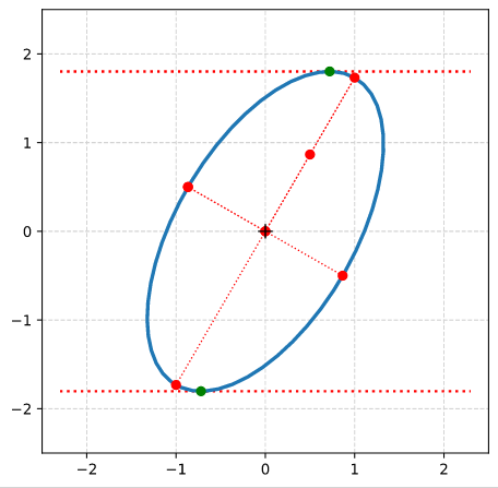
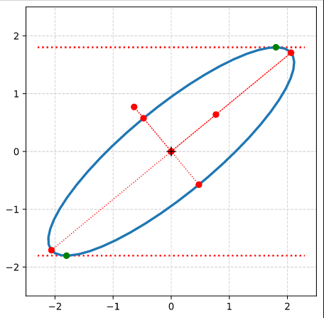
We use the example of a sheared ellipse discussed in the last post to verify the results above numerically for a 2-dim case. To write a respective Python/Numpy-program is simple. I will just give you my numerical results below.
We have used an ellipse with the longer and shorter primary axes having values a = 2 and b = 1, respectively. The ellipse was rotated by 60° against the ECS-axes.
The respective (2×2)-matrix \( \pmb{\operatorname{A}}_q^O \) had the following coefficients
\pmb{\operatorname{A}}_q^O \: = \: \begin{pmatrix} \alpha_o & 1/2\, \beta_o \\ 1/2\,\beta_o & \gamma_o \end{pmatrix} \:=\:
\begin{pmatrix} 3.25 & -1.29903811 \\ -1.29903811 & 1.75 \end{pmatrix}
\]
to fulfill
\alpha_o\,x_o^2 \, + \, \beta_o \, x_o y_o \, + \, \gamma_o \, y_o^2 \:=\: \delta_o \:=\: 4.0
\]
The shear matrix (with λS = 0.6) was
\pmb{\operatorname{M}}_{sh} \:=\: \begin{pmatrix} 1.0 & 0.6 \\ 0.0 & 1.0 \end{pmatrix}
\]
The resulting sheared ellipse became
For an ellipse we have shown that \(\pmb{\operatorname{A}}_q^S \) is given by
\pmb{\operatorname{A}}_q^S \: = \: \begin{pmatrix} \alpha_o & 1/2\,\left(\beta_o \,-\,2 \alpha_o \lambda_S \right) \\
1/2\,\left(\beta_o \,-\,2 a_o \lambda_S \right) & \alpha_o \, \lambda_S^2 \, -\, \beta_o \lambda_S \,+\, \gamma_o \end{pmatrix}
\]
From this we get the following numerical values:
A_q^S =
 [[ 3.25       -3.24903811]
 [-3.24903811  4.47884573]]
Via the Python-statement
M_sh_inv = np.linalg.inv(M_sh)
and
A_q^S_2 = M_sh_inv.T @ A_q @ M_sh_inv
we get the following values
A_q^S_2 =
 [[ 3.25       -3.24903811]
 [-3.24903811  4.47884573]]
Identical! Using
U_sh, S, Vt_sh = np.linalg.svd(M_sh, full_matrices=True)
S_sh = np.diag(S)
M_sh_2 = U_sh @ S_sh @ Vt_sh
M_sh_inv_2 = Vt_sh.T @ np.linalg.inv(S_sh) @ U_sh.T
A_q^S_2 = M_sh_inv_2.T @ A_q @ M_sh_inv_2
we also reproduce the exactly same values.
Conclusion
We have shown how a shear matrix \( \pmb{\operatorname{M}}_{sh} \) transforms the matrix \(\pmb{\operatorname{A}}_{qn}^O \) which defines an un-sheared n-dimensional ellipsoid into a matrix \(\pmb{\operatorname{A}}_{qn}^S \) defining its sheared counterpart. We have also had a glimpse on a SVD decomposition of a shear matrix. The results will enable us in the next post to apply shear operations on a concrete example of a 3-dimensional ellipsoid.