This post requires Javascript to display formulas!
In Machine Learning [ML] or statistics it is interesting to visualize properties of multivariate distributions by projecting them into 2- or 3-dimensional sub-spaces of the datas’ original n-dimensional variable space. The 3-dimensional aspects are not so often used because plotting is more complex and you have to fight with transparency aspects. Nevertheless a 3-dim view on data may sometimes be more instructive than the analysis of 2-dim projections. In this post we care about 3-dim data representations of tri-variate distributions X with matplotlib. And we add ellipsoids from a corresponding tri-variate normal distribution with the same covariance matrix as X.
Multivariate normal distribution and their projection into a 3-dimensional sub-space
A statistical multivariate distribution of data points is described by a so called random vector X in an Euclidean space for the relevant variables which characterize each object of interest. Many data samples in statistics, big data or ML are (in parts) close to a so called multivariate normal distribution [MND]. One reason for this is, by the way, the “central limit theorem”. A multivariate data distribution in the ℝn can be projected orthogonally onto a 3-dimensional sub-space. Depending on the selected axes that span the sub-space you get a tri-variate distribution of data points.
Whilst analyzing a multivariate distribution you may want to visualize for which regions of variable values your projected tri-variate distributions X deviate from adapted and related theoretical tri-variate normal distributions. The relation will be given by relevant elements of the covariance matrix. Such a deviation investigation defines an application “case 1”.
Another application case, “case 2”, is the following: We may want to study a 3-variate MND, a TND, to get a better idea about the behavior of MNDs in general. In particular you may want to learn details about the relation of the TND with its orthogonal projections onto coordinate planes. Such projections give you marginal distributions in sub-spaces of 2 dimensions. The step from analyzing bi-variate to analyzing tri-variate normal distributions quite often helps to get a deeper understanding of MNDs in spaces of higher dimension and their generalized properties.
When we have a given n-dimensional multivariate random vector X (with n > 3) we get 3-dimensional data by applying an orthogonal projection operator P on the vector data. The relatively trivial operator projects the data orthogonally into a sub-volume spanned by three selected axes of the full variable space. For a given random vector their will, of course, exist multiple such projections as there is a whole bunch of 3-dim sub-spaces for a big n. In “case 2”, however, we just create basic vectors of a 3-dim MND via a proper random generation function.
Regarding matplotlib for Python we can use a scatter-plot function to visualize the resulting data points in 3D. Typically, plots of an ideal or approximate tri-variate normal distribution [TND] will show a dense ellipsoidal core, but also a diffuse and only thinly populated outer region. To get a better impression of the spatial distribution of X relative to a TND and the orientation of the latter’s main axes it might be helpful to include ideal contour surfaces of the TND into the plots.
It is well known that the contour surfaces of multivariate normal distributions are surfaces of nested ellipsoids. On first sight it may, hower, appear difficult to combine impressions of such 2-dim hyper-surfaces with a 3-dim scatter plot. In particular: Where from do we get the main axes of the ellipsoids? And how to plot their (hyper-) surfaces?
Objective of this post
The objective of this post is to show that we can derive everything that is required
- to plot general tri-variate distributions
- plus ellipsoids from corresponding tri-variate normal distributions
from the covariance matrix Σ of our random vector X.
In case 2 we will just have to define such a matrix – and everything else will follow from it. In case 1 you have to first determine the (n x n)-covariance matrix of your random vector and then extract the relevant elements for the (3 x 3)-covariance matrix of the projected distribution out of it.
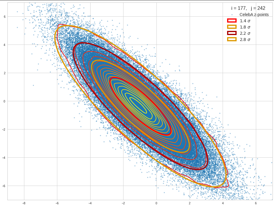
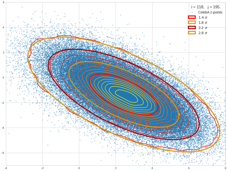
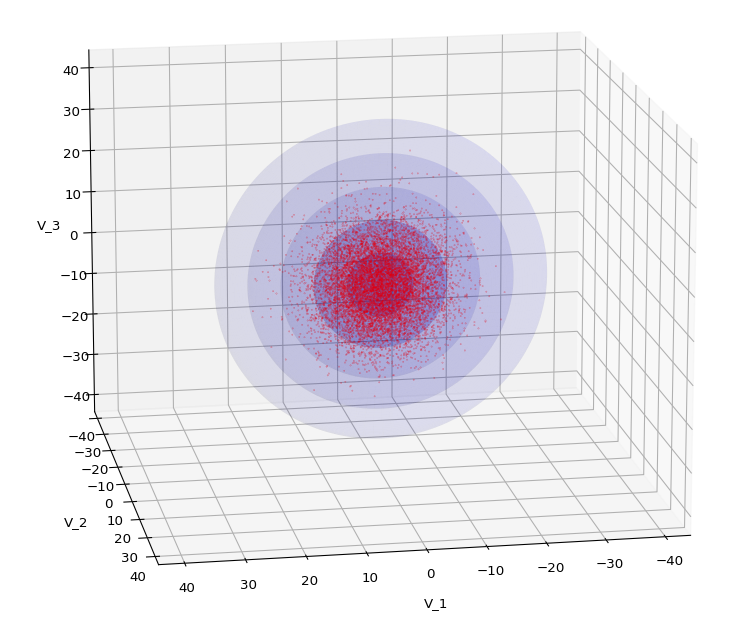
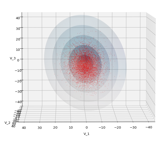
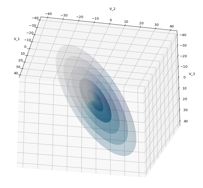
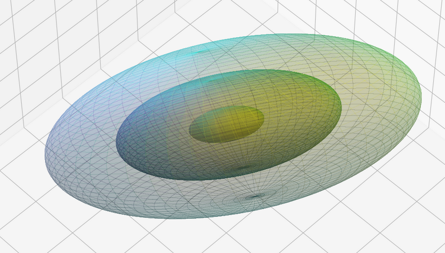
The result will be plots like the following:

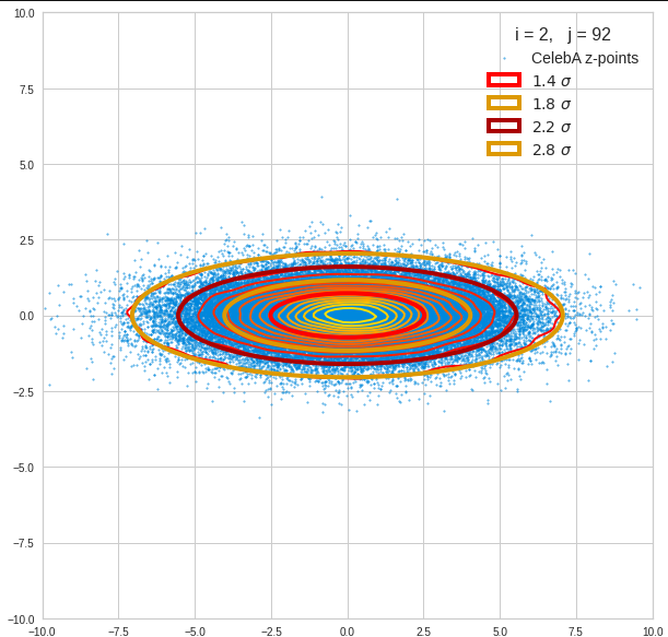
The first plot combines a scatter plot of a TND with ellipsoidal contours. The 2nd plot only shows contours for confidence levels 1 ≤ σ ≤ 5 of our ideal TND. And I did a bit of shading.
How did I get there?
The covariance matrix determines everything
The mathematical object which characterizes the properties of a MND is its covariance matrix (Σ). Note that we can determine a (n x n)-covariance matrix for any X in n dimensions. Numpy provides a function cov() that helps you with this task. The relevant elements of the full covariance matrix for orthogonal projections into a 3-dim sub-space can be extracted (or better: cut out) by applying a suitable projection operator. This is trivial: Just select the elements with the (i, i)- and (i, j)-indices corresponding to the selected axes of the sub-space. The extracted 9 elements will then form the covariance matrix of the projected tri-variate distribution.
In case 2 we just define a (3 x 3)-Σ as the starting point of our work.
Let us assume that we got the essential Σ-matrix from an analysis of our distribution data or that we, in case 2, have created it. How does a (3 x 3)-Σ relate to ellipsoidal surfaces that show the same deformation and relations of the axes’ lengths as a corresponding tri-variate normal distribution?
Creation of a MND from a standardized normal distribution
In general any n-dim MND can be constructed from a standardized multivariate distribution of independent (and consequently uncorrelated) normal distributions along each axis. I.e. from n univariate marginal distributions. Let us call the standardized multivariate distribution SMND and its random vector Z. We use the coordinate system [CS] where the coordinate axes are aligned with the main axes of the SMND as the CS in which we later also will describe our given distribution X. Furthermore the origin of the CS shall be located such that the SMND is centered. I.e. the mean vector μ of the distribution shall coincide with the CS’s origin:
\]
In this particular CS the (probability) density function f of Z is just a product of Gaussians gj(zj) in all dimensions with a mean at the origin and standard deviations σj = 1, for all j.
With z = (z1, z2, …, zn) being a position vector of a data point in the distribution, we have:
f_{\pmb{Z}} \:&=\: \pmb{\mathcal{N}}_n\left(\pmb{0}, \, \pmb{\operatorname{I}}_n \right) \:=\: \pmb{\mathcal{N}}_n\left(\pmb{\mu}=0 ,\, \pmb{\operatorname{\Sigma}}=\pmb{\operatorname{I}}_n \right)
\end{align}
\]
and in more detail
&= \, {1 \over \sqrt{(2\pi)^n} } \,
{\large e}^{ – \, {\Large 1 \over \Large 2} {\Large \sum\limits_{j=1}^n} \, {\Large z_j}^2 } \\
&=\, {1 \over \sqrt{(2\pi)^n} } \,
{\large e}^{ – \, {\Large 1 \over \Large 2} {\Large \pmb{z}^T\pmb{z}} } \end{align}
\]
The construction recipe for the creation of a general MND XN from Z is just the application of a (non-singular) linear transformation. I.e. we apply a (n x n)-matrix onto the position vectors of the data points in the ℝn. Let us call this matrix A. I.e. we transform the random vector Z to a new random vector XN by
\]
The resulting symmetric (!) covariance matrix ΣX of XN is given by
\]
Σ determines the shape of the resulting probability distribution completely. We can reconstruct an A’ which produces the same distribution by an eigendecomposition of the matrix ΣX. A’ afterward appears as a combination of a rotation and a scaling. An eigendecomposition leads in general to
\]
with V being an orthogonal matrix and D being a diagonal matrix. In case of a symmetric, positive-definite matrix like our Σ we even can get
\]
D contains the eigenvalues of Σ, whereas the columns of V are the components of the eigenvectors of Σ (in the present coordinate system). V represents a rotation and D a scaling.
The required transformation matrix T, which leads from the unrotated and unscaled SMND Z to the MND XN, can be rewritten as
\]
with
\]
The 1/2 abbreviates the square root of the matrix values (i.e. of the eigenvalues). A relevant condition is that ΣX is a symmetric and positive-definite matrix. Meaning: The original A itself must not be singular!
This works in n dimensions as well as in only 3.
Creation of a trivariate normal distribution
The creation of a centered tri-variate normal distribution is easy with Python and Numpy: We just can use
np.random.multivariate_normal( mean, Σ, m )
to create m statistical data points of the distribution. Σ must of course be delivered as a (3 x 3)-matrix – and it has to be positive definite. In the following example I have used
31 & -4 & 5 \\
-4 & 26 & 44 \\
5 & 44 & 85
\end{pmatrix}}
\]
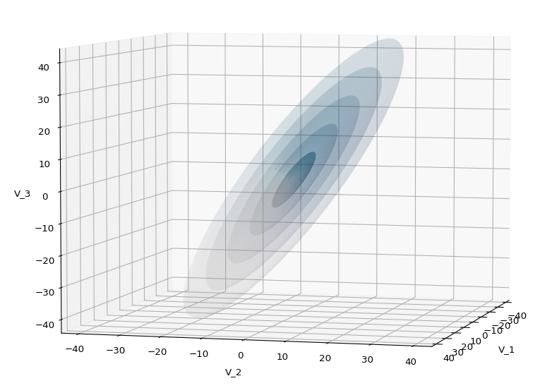
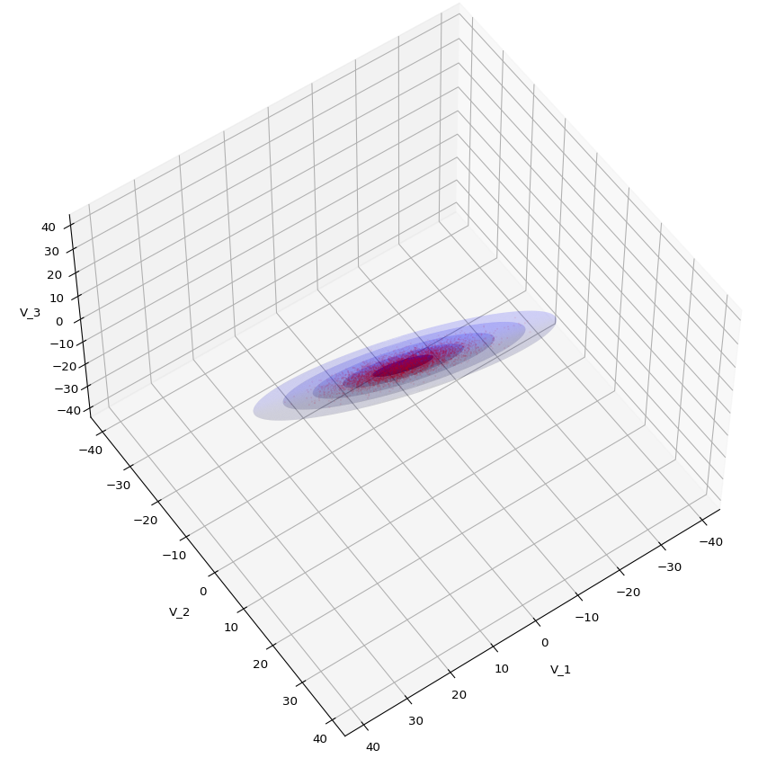
We have to feed this Σ-matrix directly into np.random.multivariate_normal(). The result with 20,000 data points looks like:
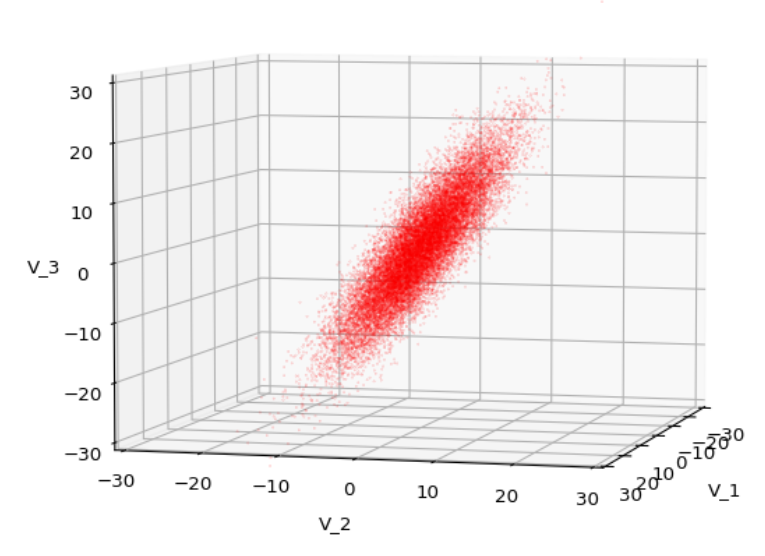
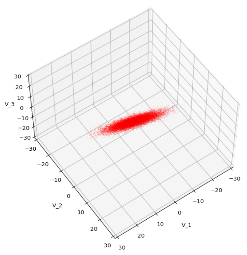
We see a dense inner core, clearly having an ellipsoidal shape. While the first image seems to indicate an overall slim ellipsoid, the second image reveals that our TND actually looks more like an extended lens with a diagonal orientation in the CS. =>
Note: When making such §D-plots we have to be careful not to make premature conclusions about the overall shape of the distribution! Projection effects may give us a wrong impression when looking from just one particular position and viewing angle onto the 3-dimensional distribution.
Create some nested transparent ellipsoidal surfaces
Especially in the outer regions the distribution looks a bit fluffy and not well defined. The reason is the density of points drops rapidly beyond a 3-σ-level. One gets the idea that a sequence of nested contour surfaces may be helpful to get a clearer image of the spatial distribution. We know already that contour surfaces of a MND are the surfaces of ellipsoids. How to get these surfaces?
The answer is rather simple: We just have to apply the mathematical recipe from above to specific data points. These data points must be located on the surface of a unit sphere (of the Z-distribution). Let us call an array with three rows for x-, y-, z-values and m columns for the amount of data points on the 3-dimensional unit sphere US. Then we need to perform the following transformation operation:
\]
to get a valid distribution SX of points on the surface of an ellipsoid with the right orientation and relation of the main axes lengths. The surface of such an ellipsoid defines a contour surface of a TND with the covariance matrix Σ.
After the application of T to these special points we can use matplotlib’s
ax.plot_surface(x, y, z, …)
to get a continuous surface image.
To get multiple nested surfaces with growing diameters of the related ellipsoids we just have to scale (with growing and common integer factors applied to the σj-eigen-values).
Note that we must create all the surfaces transparent – otherwise we would not get a view to inner regions and other nested surfaces. See the code snippets below for more details.
SVD decomposition
We also have to get serious about numerically calculating T. I.e., we need a way to perform the “eigendecomposition”. Technically, we can use the so called “Singular Value Decomposition” [SVD] from Numpy’s linalg-module, which for symmetric matrices just becomes the eigendecomposition.
Code snippets
We can now write down some Jupyter cells with Python code to realize our SVD decomposition. I omit any functionality to project your real data into a 3-dim sub-space and to derive the covariance matrix. These are standard procedures in ML or statistics. But the following code snippets will show which libraries you need and the basic steps to create your plots. Instead of a general MND, I will create a TND for scatter plot points:
Code cell 1 – Imports
import numpy as np
import matplotlib as mpl
from matplotlib import pyplot as plt
from matplotlib.colors import ListedColormap
import matplotlib.patches as mpat
from matplotlib.patches import Ellipse
from matplotlib.colors import LightSource
Code cell 2 – Function to create points on a unit sphere
# Function to create points on unit sphere
def pts_on_unit_sphere(num=200, b_print=True):

    # Create pts on unit sphere
    u = np.linspace(0, 2 * np.pi, num)
    v = np.linspace(0, np.pi, num)

    x = np.outer(np.cos(u), np.sin(v))
    y = np.outer(np.sin(u), np.sin(v))
    z = np.outer(np.ones_like(u), np.cos(v))

    # Make array
    unit_sphere = np.stack((x, y, z), 0).reshape(3, -1)

    if b_print:
        print()
        print("Shapes of coordinate arrays : ", x.shape, y.shape, z.shape)
        print("Shape of unit sphere array : ",  unit_sphere.shape)
        print()

    return unit_sphere, x
Code cell 3 – Function to plot TND with ellipsoidal surfaces
# Function to plot a TND with supplied allipsoids based on the sam Sigma-matrix
def plot_TND_with_ellipsoids(elevation=5, azimuth=5,
                             size=12, dpi=96,
                             lim=30, dist=11,
                             X_pts_data=[],
                             li_ellipsoids=[],
                             li_alpha_ell=[],
                             b_scatter=False, b_surface=True,
                             b_shaded=False, b_common_rgb=True,
                             b_antialias=True,
                             pts_size=0.02, pts_alpha=0.8,
                             uniform_color='b', strid=1,
                             light_azim=65, light_alt=45
                            ):

    # Prepare figure
    plt.rcParams['figure.dpi'] = dpi
    fig = plt.figure(figsize=(size,size))  # Square figure
    ax = fig.add_subplot(111, projection='3d')

    # Check data
    if b_scatter:
        if len(X_pts_data) == 0:
            print("Error: No scatter points available")
            return

    if b_surface:
        if len(li_ellipsoids) == 0:
             print("Error: No ellipsoid points available")
             return
        if len(li_alpha_ell) < len(li_ellipsoids):
             print("Error: Not enough alpha values for ellipsoida")
             return
        num_ell = len(li_ellipsoids)

    # set limits on axes
    if b_surface:
        lim = lim * 1.7
    else:
        lim = lim

    # axes and labels
    ax.set_xlim(-lim, lim)
    ax.set_ylim(-lim, lim)
    ax.set_zlim(-lim, lim)
    ax.set_xlabel('V_1', labelpad=12.0)
    ax.set_ylabel('V_2', labelpad=12.0)
    ax.set_zlabel('V_3', labelpad=6.0)

    # scatter points of the MND
    if b_scatter:
        x = X_pts_data[:, 0]
        y = X_pts_data[:, 1]
        z = X_pts_data[:, 2]
        ax.scatter(x, y, z, c='r', marker='o', s=pts_size, alpha=pts_alpha)

    # ellipsoidal surfaces
    if b_surface:
        # Shaded
        if b_shaded:
            # Light source
            ls = LightSource(azdeg=light_azim, altdeg=light_alt)
            cm = plt.cm.PuBu
            li_rgb = []
            for i in range(0, num_ell):
                zz = li_ellipsoids[i][2,:]
                li_rgb.append(ls.shade(zz, cm))

            if b_common_rgb:
                for i in range(0, num_ell-1):
                    li_rgb[i] = li_rgb[num_ell-1]

            # plot the ellipsoidal surfaces
            for i in range(0, num_ell):
                ax.plot_surface(*li_ellipsoids[i],
                                rstride=strid, cstride=strid,
                                linewidth=0, antialiased=b_antialias,
                                facecolors=li_rgb[i],
                                alpha=li_alpha_ell[i]
                               )
        # just uniform color
        else:
            print("here")
            #ax.plot_surface(*ellipsoid, rstride=2, cstride=2, color='b', alpha=0.2)
            for i in range(0, num_ell):
                ax.plot_surface(*li_ellipsoids[i],
                                rstride=strid, cstride=strid,
                                color=uniform_color, alpha=li_alpha_ell[i])

    ax.view_init(elev=elevation, azim=azimuth)
    ax.dist = dist
    return
Some hints: The scatter data from the distribution X (or XN) must be provided as a Numpy array. The TND-ellipsoids and the respective alpha values must be provided as Python lists. Also the size and the alpha-values for the scatter points can be controlled. Reducing both can be helpful to get a glimpse also on ellipsoids within the relative dense core of the TND.
Some parameters as “elevation”, “azimuth”, “dist” help to control the viewing perspective. You can switch showing of the scatter data as well as ellipsoidal surfaces and their shading on and off by the Boolean parameters.
There are a lot of parameters to control a primitive kind of shading. You find the relevant information in the online documentation of matplotlib. The “strid” (stride) parameter should be set to 1 or 2. For slower CPUs one can also take higher values. One has to define a light-source and a rgb-value range for the z-values. You are free to use a different color-map instead of PuBu and make that a parameter, too.
Code cell 4 – Covariance matrix, SVD decomposition and derivation of the T-matrix
b_print = True

# Covariance matrix
cov1 = [[31.0, -4, 5], [-4, 26, 44], [5, 44, 85]]
cov = np.array(cov1)

# SVD Decomposition
U, S, Vt = np.linalg.svd(cov, full_matrices=True)
S_sqrt = np.sqrt(S)

# get the trafo matrix T = U*SQRT(S)
T = U * S_sqrt

# Print some info
if b_print:
    print("Shape U: ", U.shape, " :: Shape S: ", S.shape)
    print(" S      : ", S)
    print(" S_sqrt : ", S_sqrt)
    print()
    print(" U :\n", U)
    print(" T :\n", T)
Code cell 5 – Transformation of points on a unit sphere
# Transform pts from unit sphere onto surface of ellipsoids
# ~~~~~~~~~~~~~~~~~~~~~~~~~~~~~~~
b_print = True
num = 200
unit_sphere, xs = pts_on_unit_sphere(num=num)

# Apply transformation on data of unit sphere
ell_transf = T @ unit_sphere
# li_fact = [2.5, 3.5, 4.5, 5.5, 6.5]
li_fact = [1.0, 2.0, 3.0, 4.0, 5.0]
num_ell = len(li_fact)
li_ellipsoids = []
for i in range(0, num_ell):
    li_ellipsoids.append(li_fact[i] * ell_transf.reshape(3, *xs.shape))

if b_print:
    print("Shape ell_transf  : ", ell_transf.shape)
    print("Shape ell_transf0 : ", li_ellipsoids[0].shape)
Code cell 6 – TND data point creation and plotting
# Create TND-points
n = 10000
mean=[0,0,0]
pts_data = np.random.multivariate_normal(mean, cov1, n)

# Alpha values for the ellipsoids
common_alpha = 0.05
li_alpha_ell = []
for i in range(0, num_ell):
    li_alpha_ell.append(common_alpha)
#li_alpha_ell = [0.08, 0.05, 0.05, 0.05, 0.05]
#li_alpha_ell = [0.12, 0.1, 0.08, 0.08, 0.08]
li_alpha_ell = [0.3, 0.1, 0.08, 0.08, 0.08]

# Plotting
elev = 5
azim = 15
plot_TND_with_ellipsoids(elevation=elev, azimuth=azim,
                         lim= 25, dist=11,
                         X_pts_data = pts_data,
                         li_ellipsoids=li_ellipsoids,
                         li_alpha_ell=li_alpha_ell,
                         b_scatter=True, b_surface=True,
                         b_shaded=False, b_common_rgb=False,
                         b_antialias=True,
                         pts_size=0.018, pts_alpha=0.6,
                         uniform_color='b', strid=2,
                         light_azim=65, light_alt=75
                       )
#
Example views
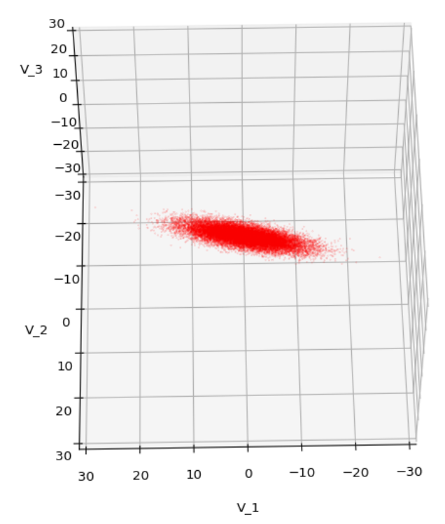
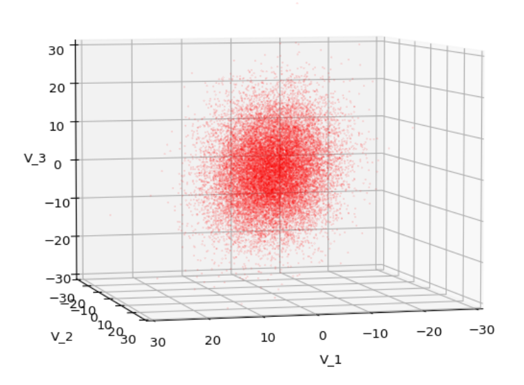
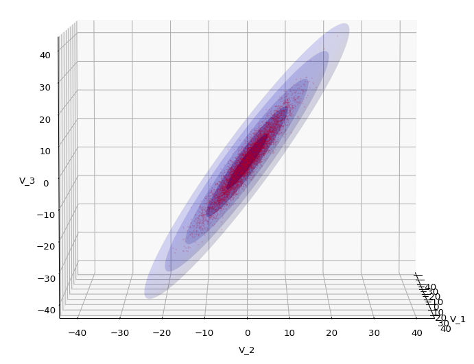
Let us play a bit around. The ellipsoidal contours are for σ = 1, 2, 3 ,4, 5. First we look at the data distribution from above. The ellipsoidal contours are for σ = 1, 2, 3 ,4, 5. We must reduce the size and alpha of the scatter points to 0.01 and 0.45, respectively, to still get an indication of the innermost ellipsoid of σ = 1. I used 8000 scatter points. The following plots show the same from different side perspectives – with and without shading and adapted alpha-values and number values for the scatter points
 .
.
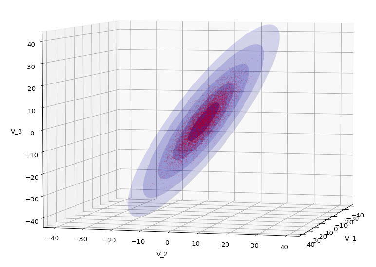
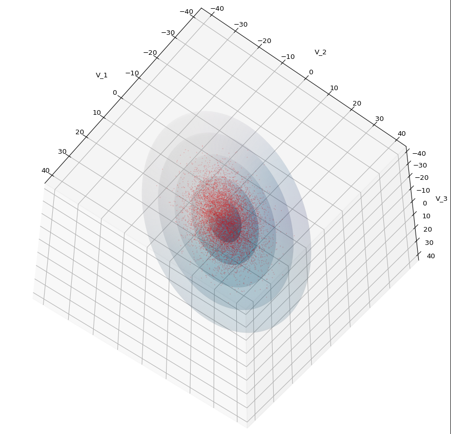
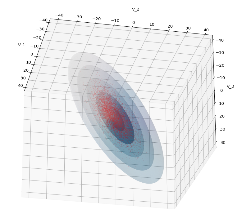
Yoo see: How a TND appears depends strongly on the viewing position. From some positions the distribution’s projection of the viewer’s background plane may even appear spherical. But on the other side it is remarkable how well the projection onto a background plane keeps up the ellipses of the projected outermost borders of the contour surfaces (of the ellipsoids for confidence levels). This is a dominant feature of MNDs in general.
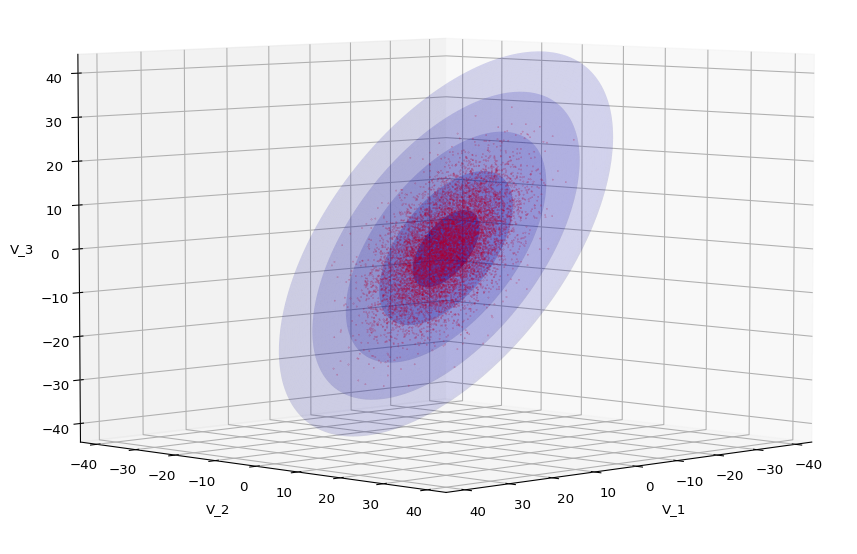
A last hint: To get a more volumetric impression it is required to both work with the position of the lightsource, the alpha-values and the colormap. In addition turning off ant-aliasing and setting the stride to something like 5 may be very helpful, too. The next image was done for an ellipsoid with slightly different extensions, only 3 ellipsoids and stride=5:
Conclusion
In this blog I have shown that we can display a tri-variate (normal) distribution, stemming from a construction of a standardized normal distribution or from a projection of some real data distribution, in 3D with the help of Numpy and matplotlib. As soon as we know the covariance matrix of our distribution we can add transparent surfaces of ellipsoids to our plots. These are constructed via a linear transformation of points on a unit sphere. The transformation matrix can be derived from an eigendecomposition of the covariance matrix.
The added ellipsoids help to better understand the shape and orientation of the tri-variate distribution. But plots from different viewing angles are required.