In my last post
Blender – complexity inside spherical and concave cylindrical mirrors – I – some impressions
I briefly discussed some interesting sculptures and optical experiments in reality. The basic ideas are worth some optical experiments in the virtual ray-tracing world of Blender. In this post I start with my trial to reconstruct something like the so called “S-curve” of the artist Anish Kapoor with Blender meshes.
If you looked at the link I gave in my last article or googled for other pictures of the S-curve you certainly saw that the metallic surface the artist placed at the Kistefoss museum is not just a simple combination of mirrored cylindrical surfaces. It is much more elegant:
The first point is that it consists of one continuous coherent piece of metal. The surface is deformed and changes its curvature continuously. It shows symmetry and rotational axes. When my wife and I first saw it we stood at a rather orthogonal position opposite of it. We only got aware of the different cylindrical deformations on the left and right side. We wondered what Kapoor had done at the middle vertical axis as we expected a gap there. Later we went to another position – and there was no gap at all, but a smooth variation of curvatures along the main axes of the object.
The second point is the combination of different curvatures: a cylindrical curvature in vertical direction (mirrored in left/right direction) plus the elegant S-like curvature in horizontal direction. The curvature in vertical direction grows with horizontal distance from the center – it is zero at the central vertical axis. The left and right part of the object are identical – they reflect a 180 °ree; rotation (not a mirroring process) around the central vertical axis. Actually, the gradient at the central rotational axis and the along the horizontal symmetry axes disappears. And no curvature at all at the central vertical axis.
All in all a lot of different symmetries and smooth curvature transitions! The artist plays with the appeal of symmetries to the human brain. But, at the same time, he breaks symmetry strongly in the visual impression of the viewer with the help of the rules of optics. Wonderful!
In this article I want to tackle the problem of a smooth transition between two cylindrically deformed surfaces in Blender first. The S-curvature is the topic of the next post.
The result first
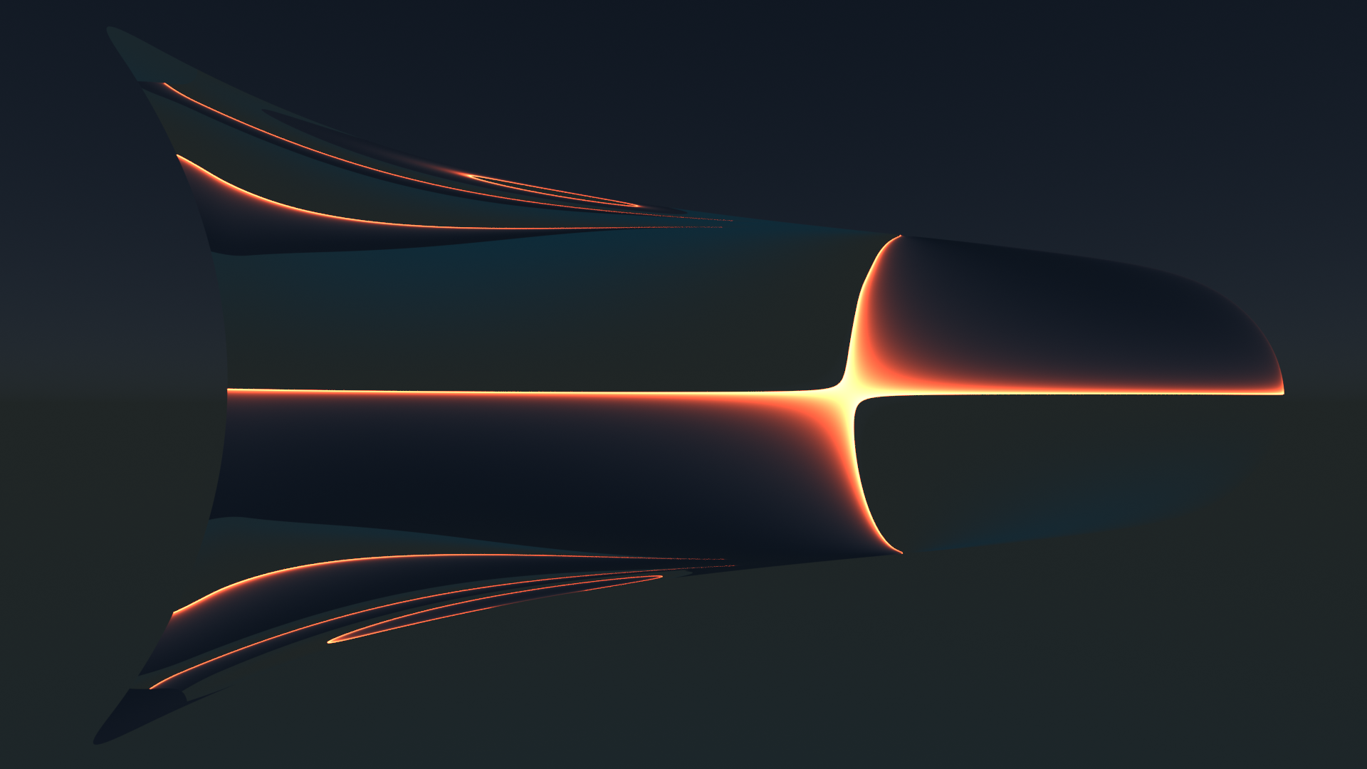
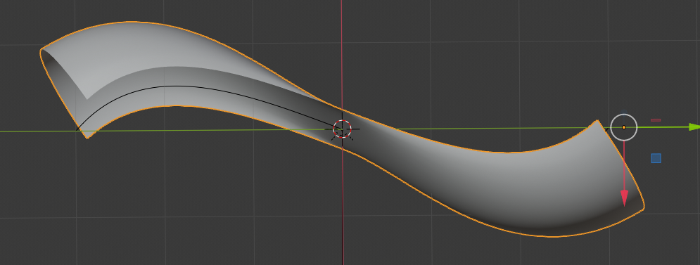
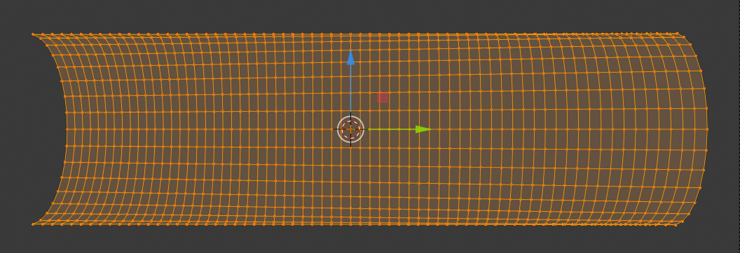
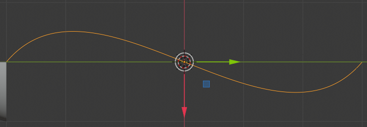
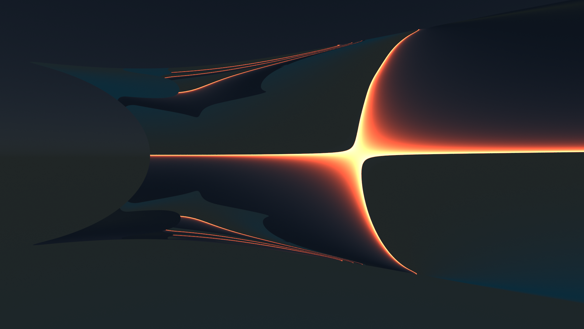
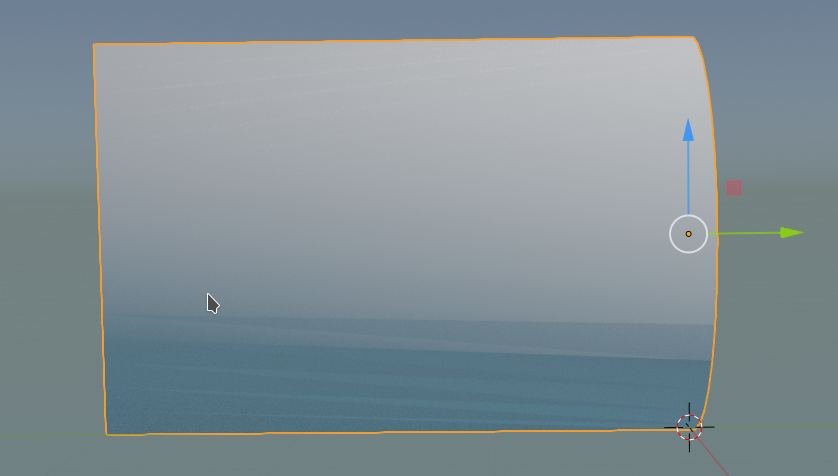
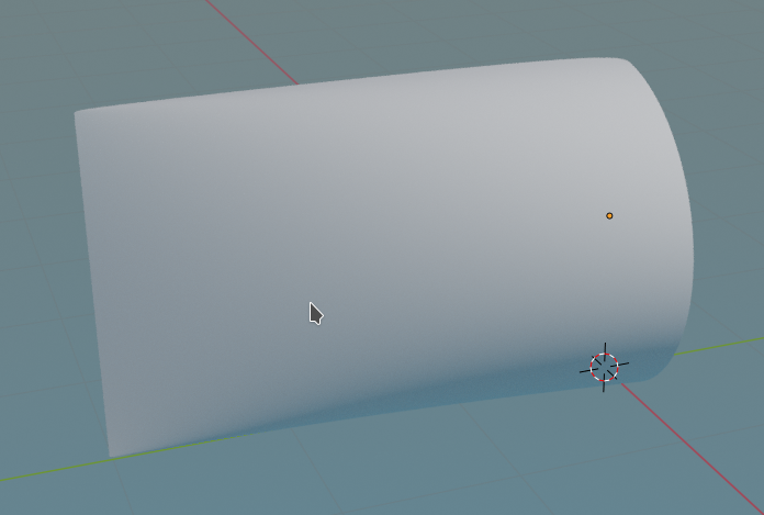
I first show you what we want to achieve:
We get an impression of the mirroring effects in “viewport shading mode” by adding a sky texture to the world background and a simple textured plane:
The reader may have detected small dips (indentations) at the centers of the upper and lower edge. I come to this point later on. Compared to the real S-curve a major difference in vertical direction is that Kapoor did not use a the full curvature of a half cylinder at the outmost left and right ends. He maybe took only a cut off part of a half circle there. But what part of a half-circle you use in the end is a minor point regarding the general construction of such a surface in Blender.
How to get there?
As I only use Blender seldom I
really wondered how to create a surface like the one shown above. Mesh based or nurbs based? And how to get a really smooth surface? Regarding the latter point you may think of subdivisions, but this is a wrong approach as a subdivision of a mesh intersects linear connections between vertices. Therefore, if you applied simple subdivision to the object you would create points not residing on a circle/cylinder/surface – which in the end would disturb the optics by visible lines and flat planes. Even if you added a smoothing modifier afterward.
The solution in the end was simple and mesh based. There is one important point to note which has to do with rules for object creation in Blender:
You define the resolution of the mesh(es) we are going to construct in the beginning!
As we need to edit some vertex positions manually the resolution in first experiments should rather be limited. For a continuous surface we shall apply a surface smoothing modifier anyway. This modifier rounds up edges a bit – which leads to the “dips” I mentioned. They will be smaller the higher you choose the meshes’ resolution – but this is something for a final polished version.
Constructional steps
All in all there are many steps to follow. I only give a basic outline. Read the Blender manual for details.
Note: I added the application of a modifier in the middle of the steps for illustration purposes. You should skip this step and apply the modifier only in the end. I sometimes experienced strange effects when applying and deleting the modifier during work with vertices.
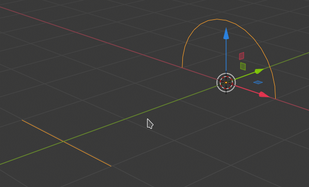
Step 1: You first create a mesh based circle. You now decide which number of mesh nodes and basic resolution of the later surface you want to have. This is done by the the tool menu that opens in Blender version 2.82 in the lower left of the viewport. Lets keep to the standard value of 32 mesh points (vertices). This obviously means that a half-circle later on will contain 17 vertices. All vertices of our first reside exactly on the circle line. The circles center resides at the global world center. You also see that 4 points of the circle sit on the world axes X, Y. Leave the circle exactly where it is. Do not apply any translation. (It would be hard to realign it with world axes later on.)
Step 2: Change to Edit mode and remove one side of the circle (left of the X-axis) by eliminating the superfluous vertices. Do it such that the end points of the remaining half-circle reside exactly on the X-axis of the world mesh. Keep the origin of the mesh were it is. Do NOT close the circle mesh on the X-axis, i.e. do not create a closed loop of vertices!
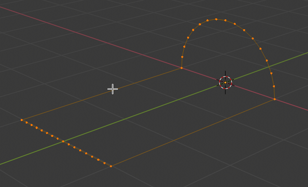
Step 3: You then add a line mesh in Object mode. This can e.g. achieved by first creating a path. Move it along the world Y-axis to get some X-distance from the half-circle (-3m). Select the path by right clicking and convert the path to a mesh by the help of a menu point. Go to Edit mode again and eliminate vertices (or adding by subdividing) – until the resulting line mesh has exactly the same number of vertices (17) as your half circle (including the end points). In object mode set the origin to the mesh’s geometry, i.e. its center. Move the line mesh to X=0. Change its X-dimension to the same value the half circle has (2m).
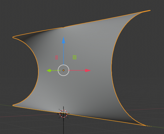
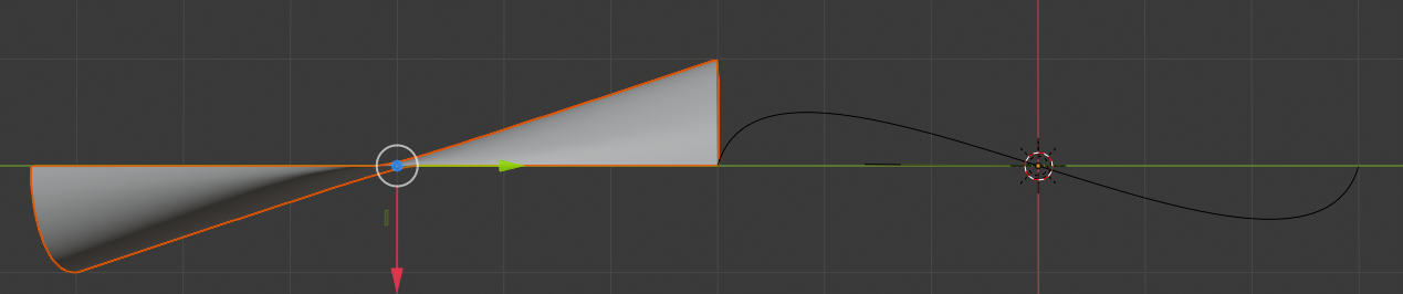
Step 4: Rotate the half-circle by 90 degrees around the X-axis to get a basic scene like in the picture below. Join the two meshes to one object.
Step 5: Go to Edit mode and provide missing edges to connect the line segment with the half-circle.
Step 6: Add faces by selecting all vertices and choosing menu point “Face > Grid Fill”.
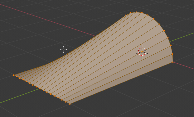
Hey, this was a major step. save your results – and make a backup copy for later experiments.
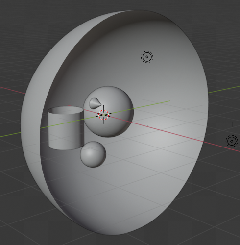
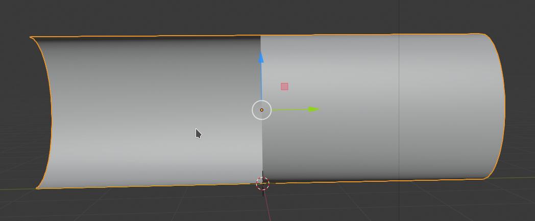
Step 7: Add a Sky Texture to the world. Activate the Cycles renderer. Rotate the object by 90 degree around the Y-axis. Choose viewport shading mode.
Step 8: Move object to Z=1m. Right click in Object mode on your object it; choose “Shade smooth”.
Just to find that you still see the edges of the faces. Smooth is not really smooth, unfortunately.
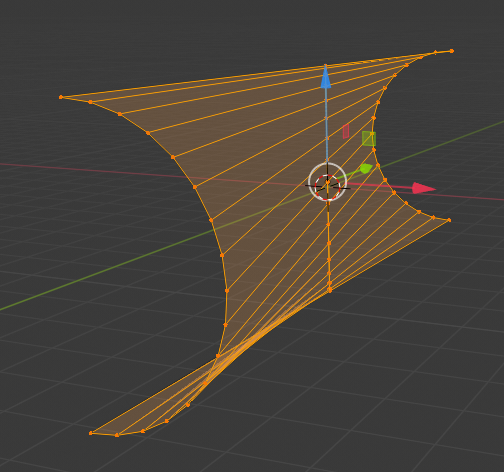
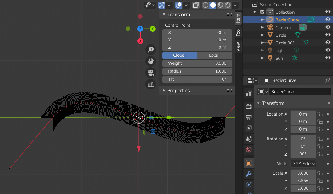
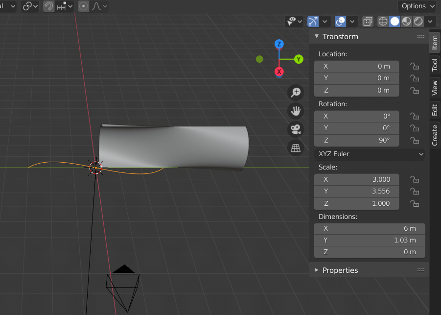
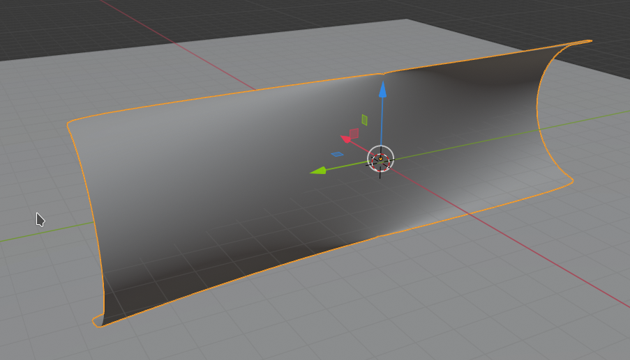
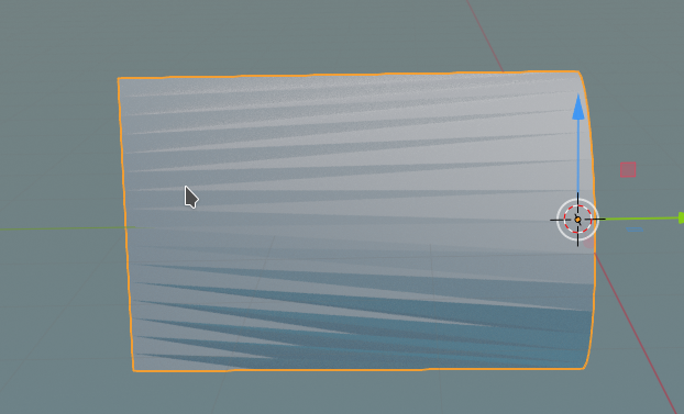
Step 9: Skip this step in your own experiment and perform it at the end of our construction. Just for illustrating that the flat surfaces can be eliminated later on, I add a modifier to our object – namely the modifier “subdivision surface” – which offers a more intelligent algorithm than “Shade smooth”. Just for testing I give it the following parameters:
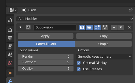
We get:
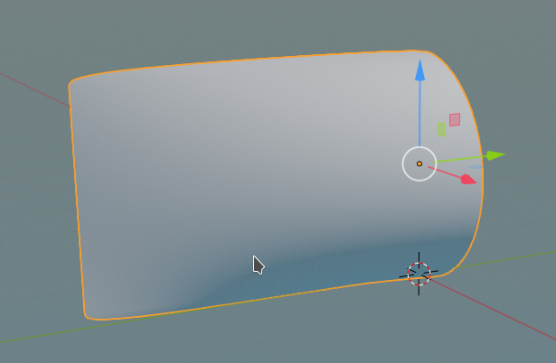
Much more convincing! You see e.g. at the left side that the corners have been rounded – this will later lead to the dips I mentioned.
Intermediate consideration
We could now duplicate our object, rotate the duplicate and join it with the original. But before we do this we change the height values of the vertices along the left edge (actually a line segment). From our construction it is clear that corresponding vertices on the half circle and the left edge cannot have the same Z-coordinate values – they reside at different heights above the ground. The “catmull clark” algorithm of our modifier therefore creates a surface with gradients and curvature varying in all coordinate directions. There is no real problem with this. However, we reduce the chance for certain caustics and cascades of multiple reflections on the concave side of the final surface. Cylindrical surfaces (i.e. with constant curvature) give rise to sharp reflective caustics. To retain a bit of this and keep the curvature rather constant in Z-direction (whilst varying in X-direction), we are going to adjust the heights of the vertices along the straight left edge to the heights of the vertices along the half-circle.
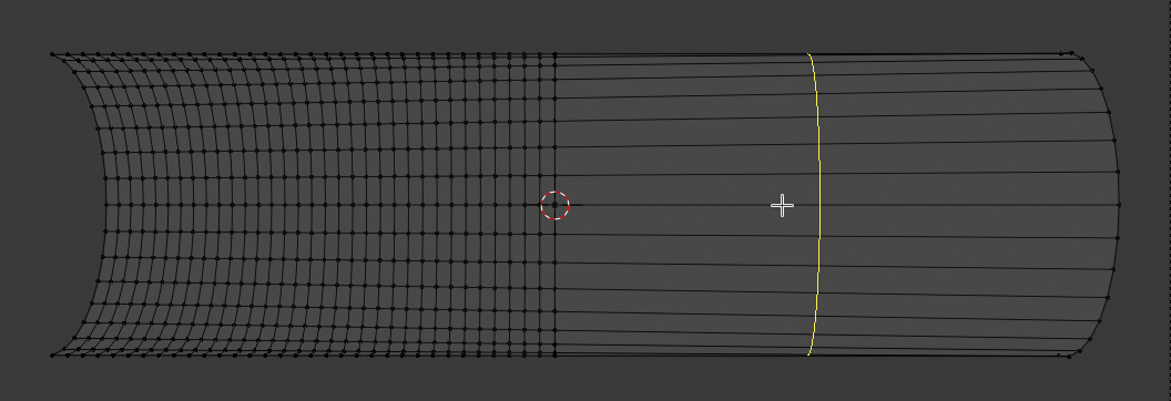
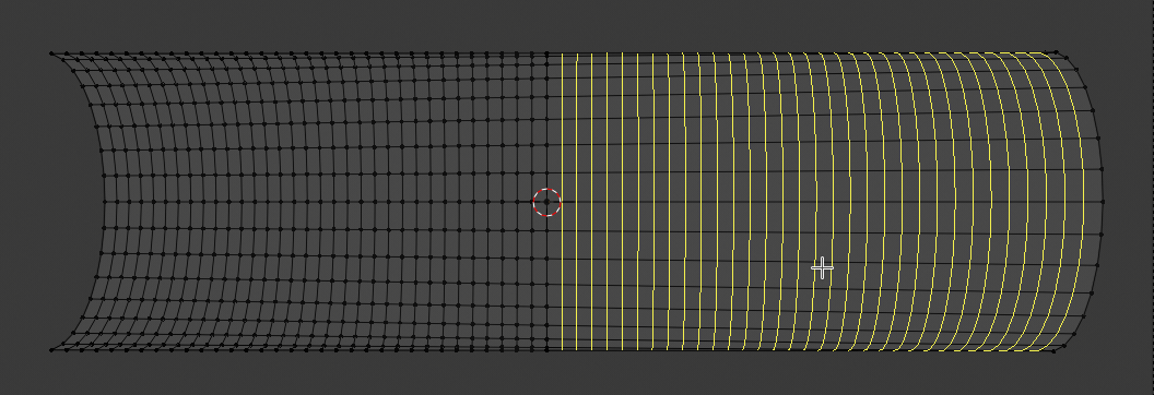
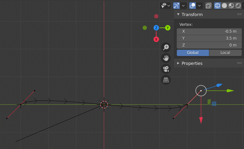
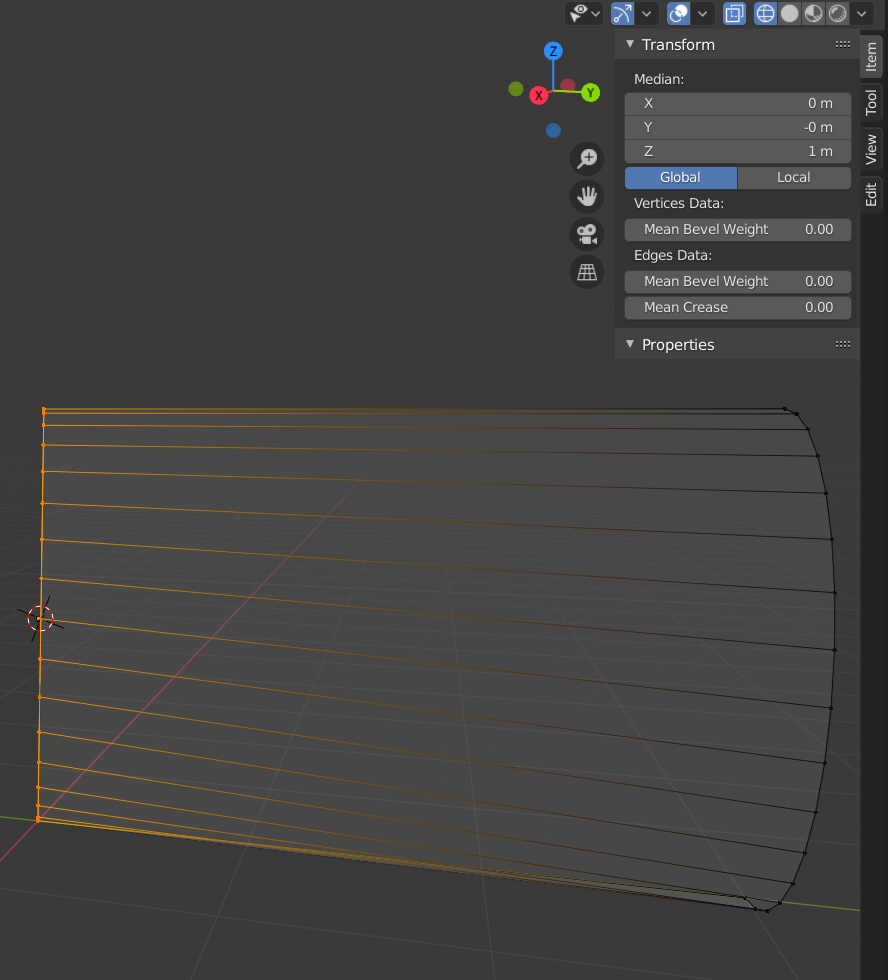
Step 10: Go to edit mode. Do NOT move the vertices of the half circle! Check the Z-value of each of the vertices of the half-circle by selecting one by one and looking at the information on
the sidebar of the Blender interface (View > Sidebar). Change the Z-coordinate of the half-circle’s counterpart on the left straight edge to the very same value. Repeat this process for all vertices of the half-circle and the corresponding ones of the straight edge.
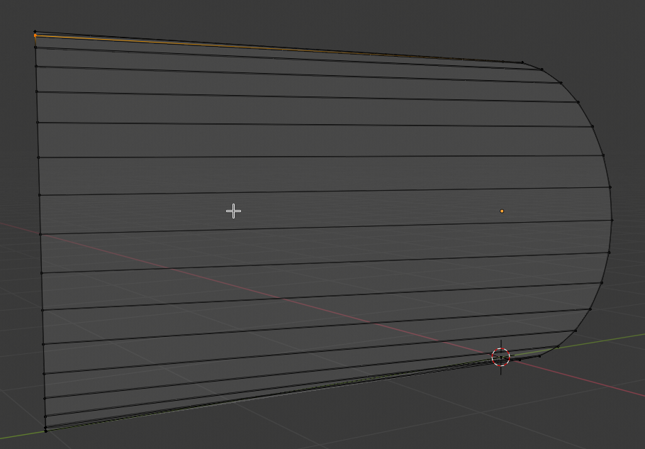
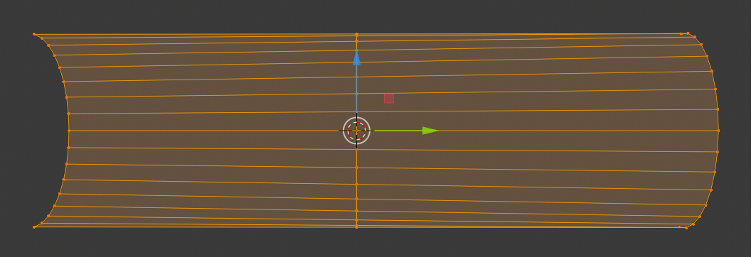
You see that the vertices are now non-equidistantly distributed along the Z-axis on the left side !
This gives us already a slightly different shading in the lower part.
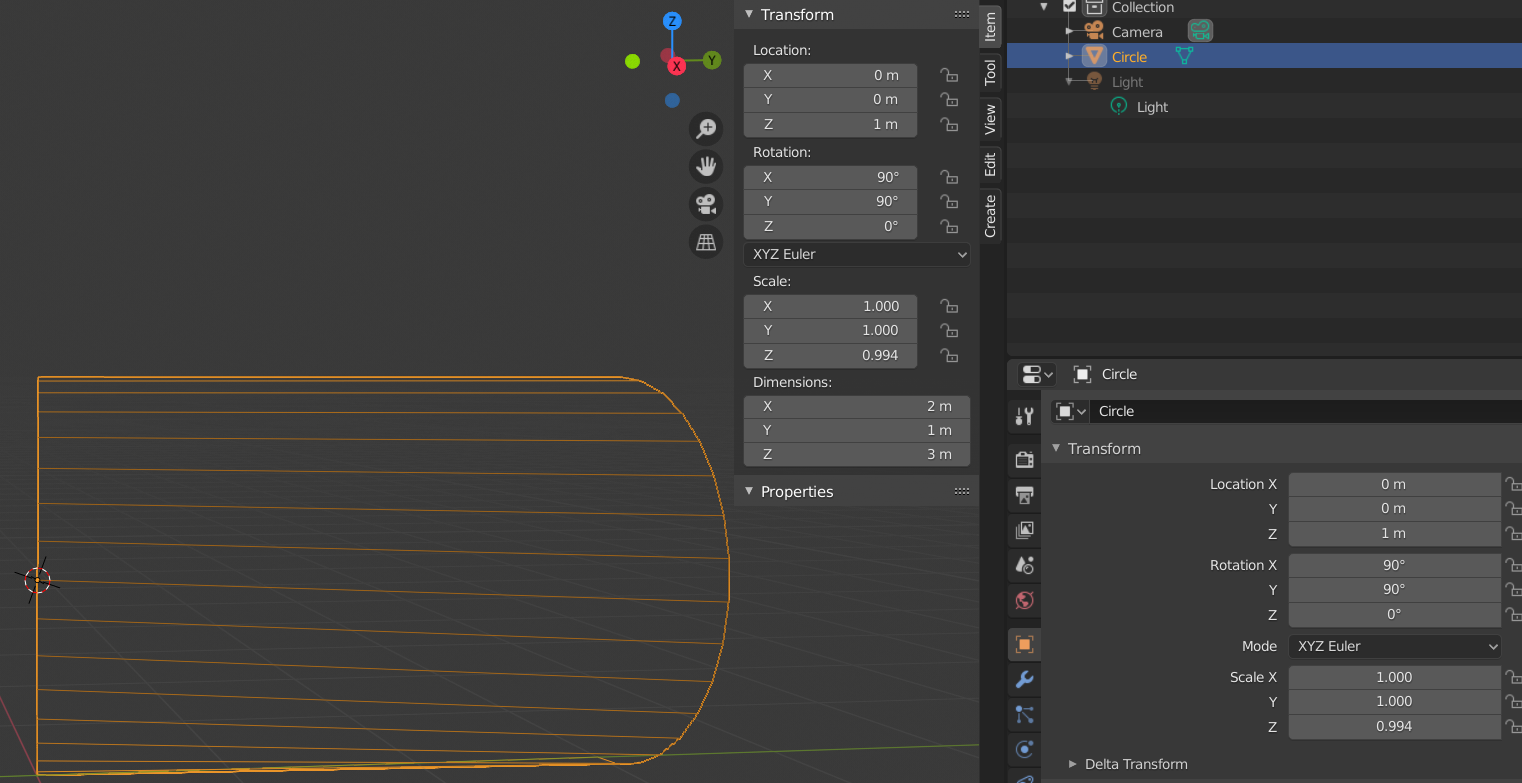
Step 11: Important! Remove the modifier if you applied it. Then: Move the object such that all vertices on the left corner are at Y=0 and X=0. For Y=0 you can just adjust the median of the vertices. Check also that the corners of the half-circle have X=0 and Y=3. All vertices of the half circle should have Y=3.
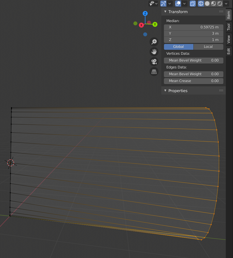
Then snap the cursor to the grid at X=0, Y=0, Z=1. Afterward snap the origin of the object to the cursor. The object’s coordinates should now be X=0, Y=0, Z=1.
Step 10: In Object mode: Duplicate the object by SHIFT D + Enter. Do not move the mouse in between; don’t touch it. Rotate the active duplicate around the Z-axis by 180 degrees.
Check the coordinates of the vertices of the mirrored object. If its right vertices reside at y=0 and its left at y=-3 then join the two objects to one. Note: At the middle there are still two rows of vertices. But their vertices should coincide exactly at their x=0, Y=0 and Z-values. If not you will see it later by some distortions in the optics.
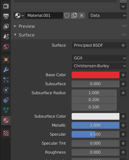
Step 11: Add a metallic material
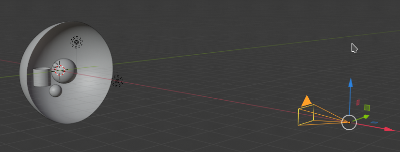
Place the camera at
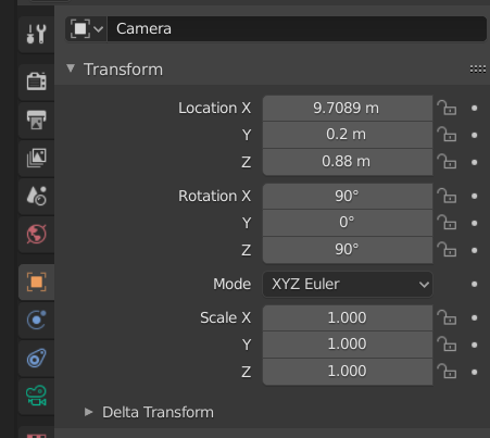
and add
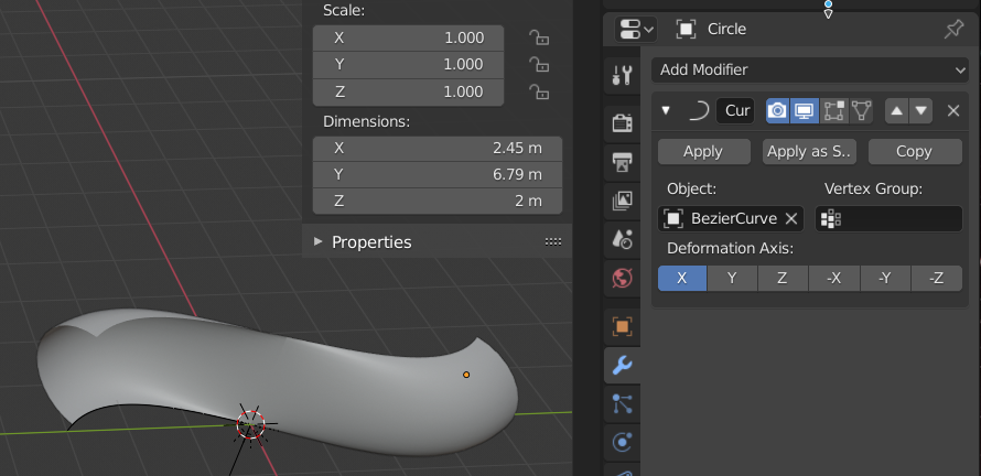
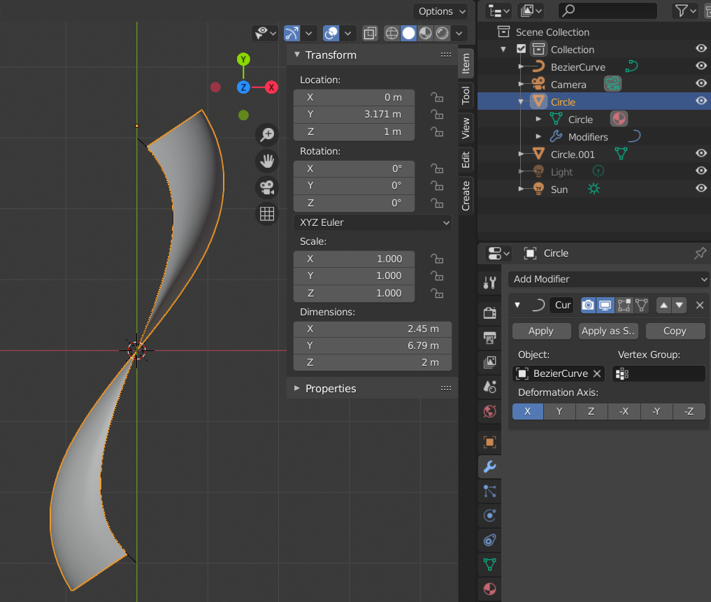
the modifier again with the settings given above. Render with the help of the material preview:
Step 11: Add a Sun at almost 180 degrees and play a bit with the sky
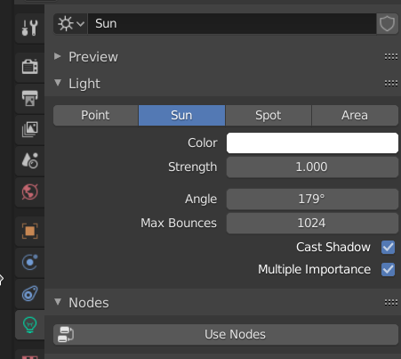
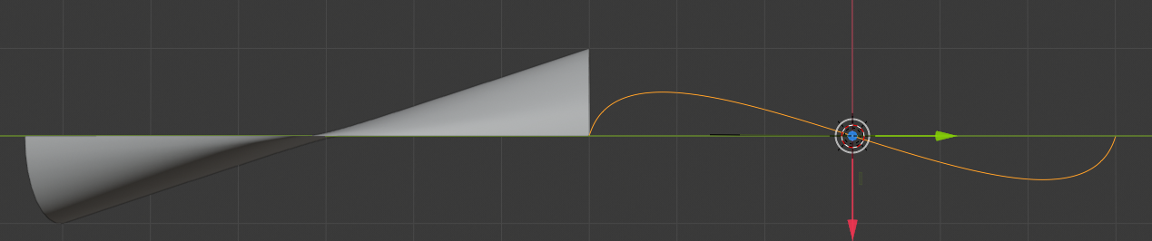
We get in full viewport shading:
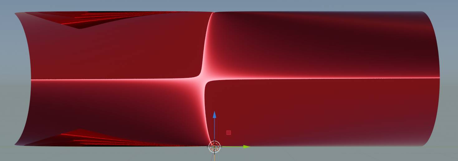
Watch the sharp edges created by multi-reflections on the left concave side of the object. This we got due to our laborious adjustment of the Z-coordinates of our central vertices.
Save your result for later purposes!
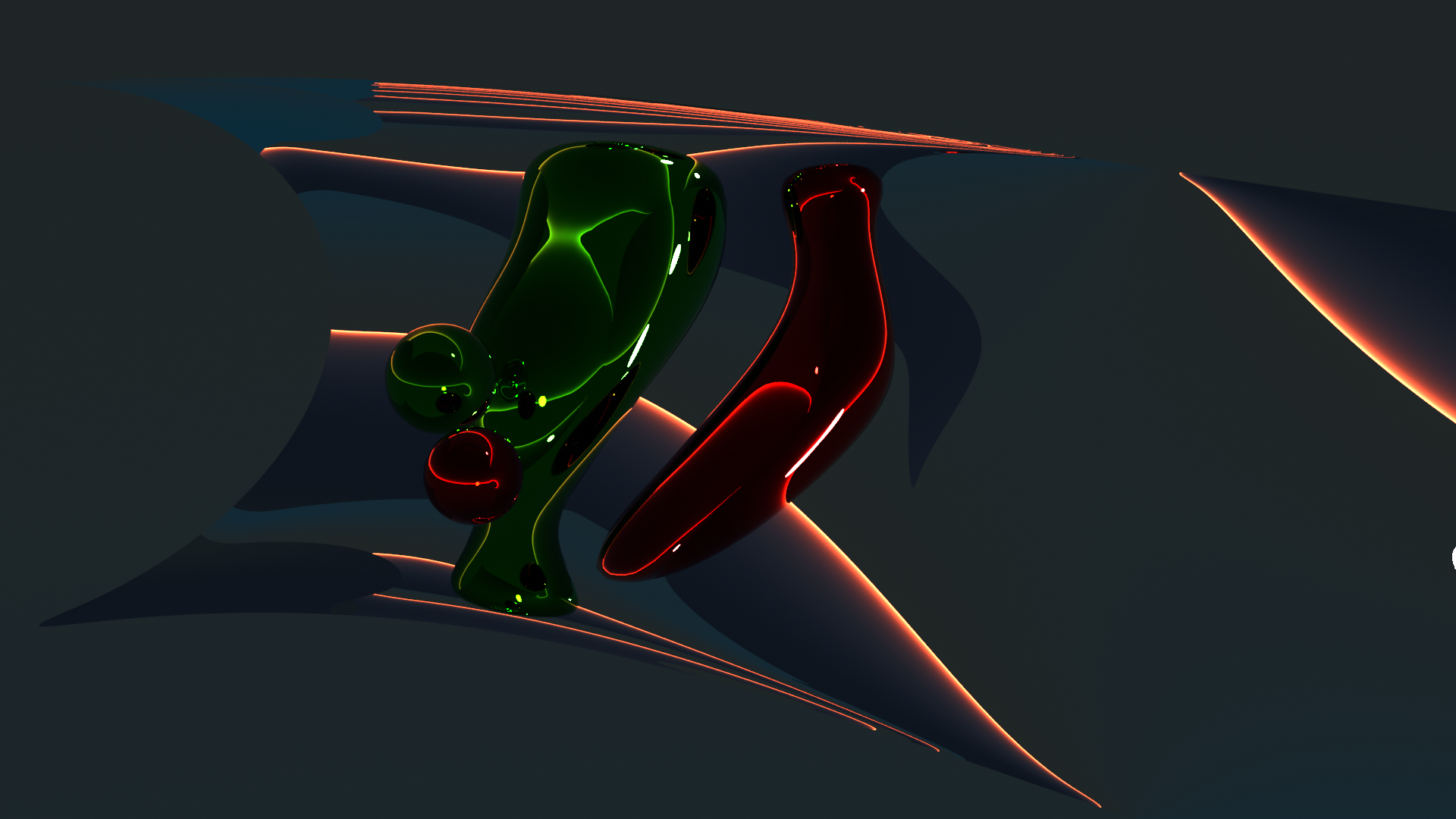
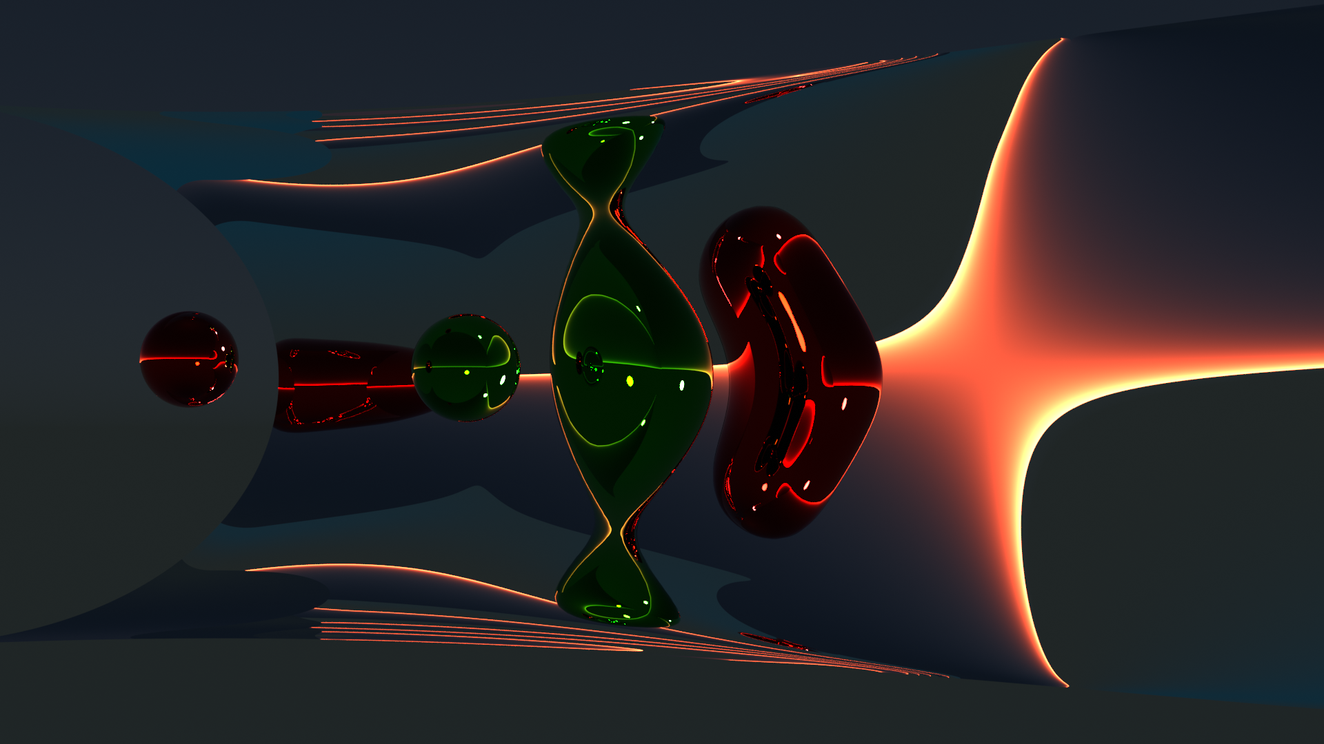
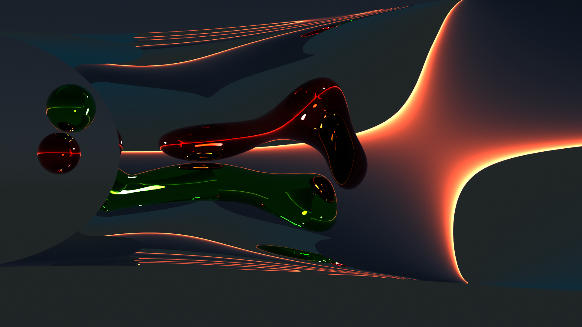
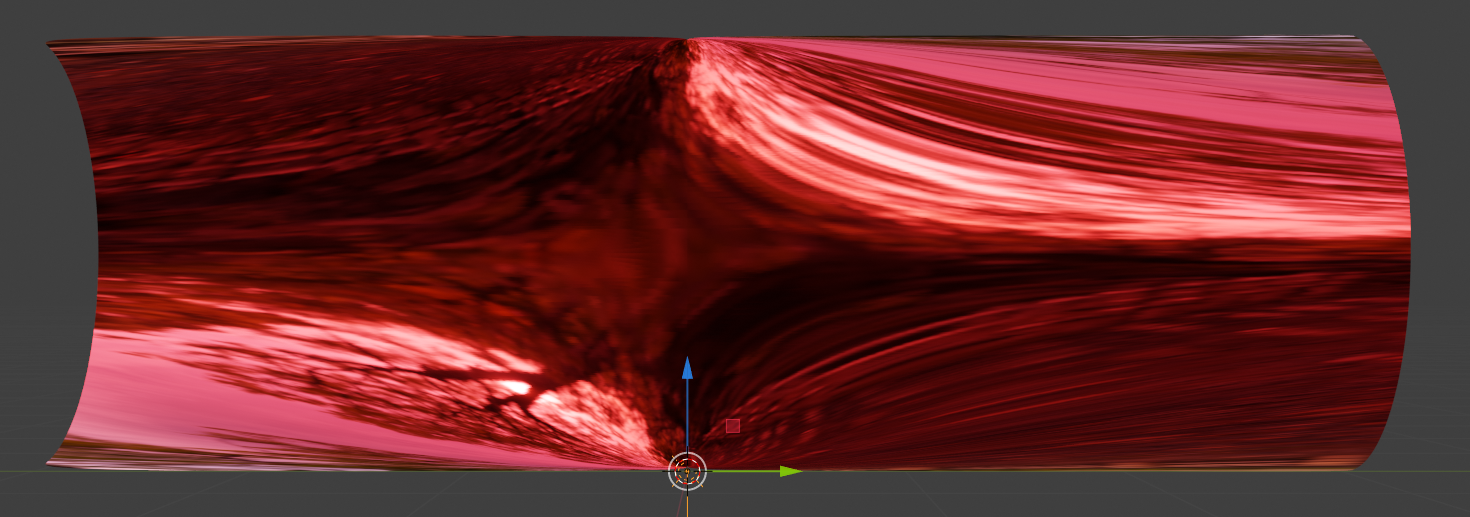
Adding some elements to the scene
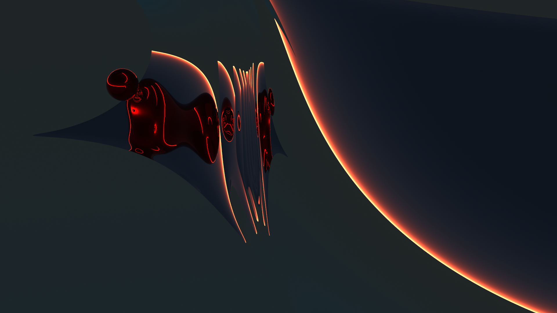
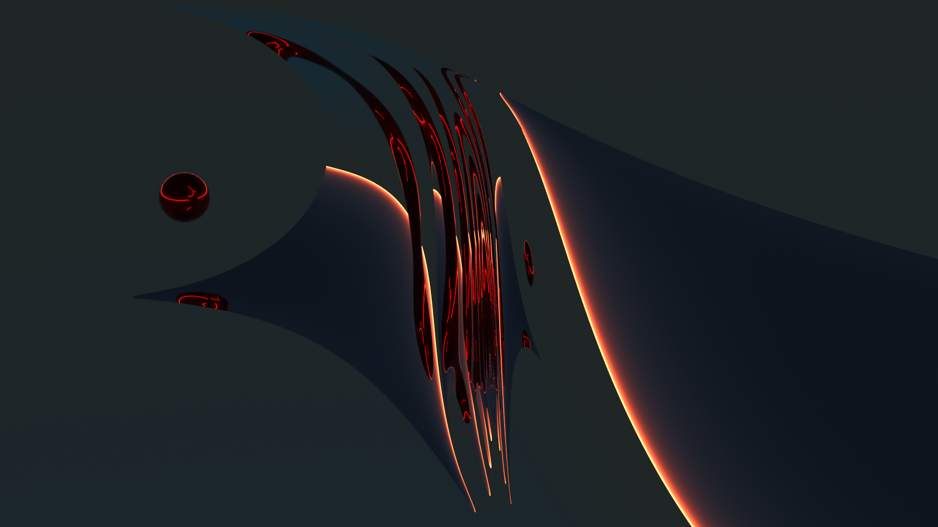
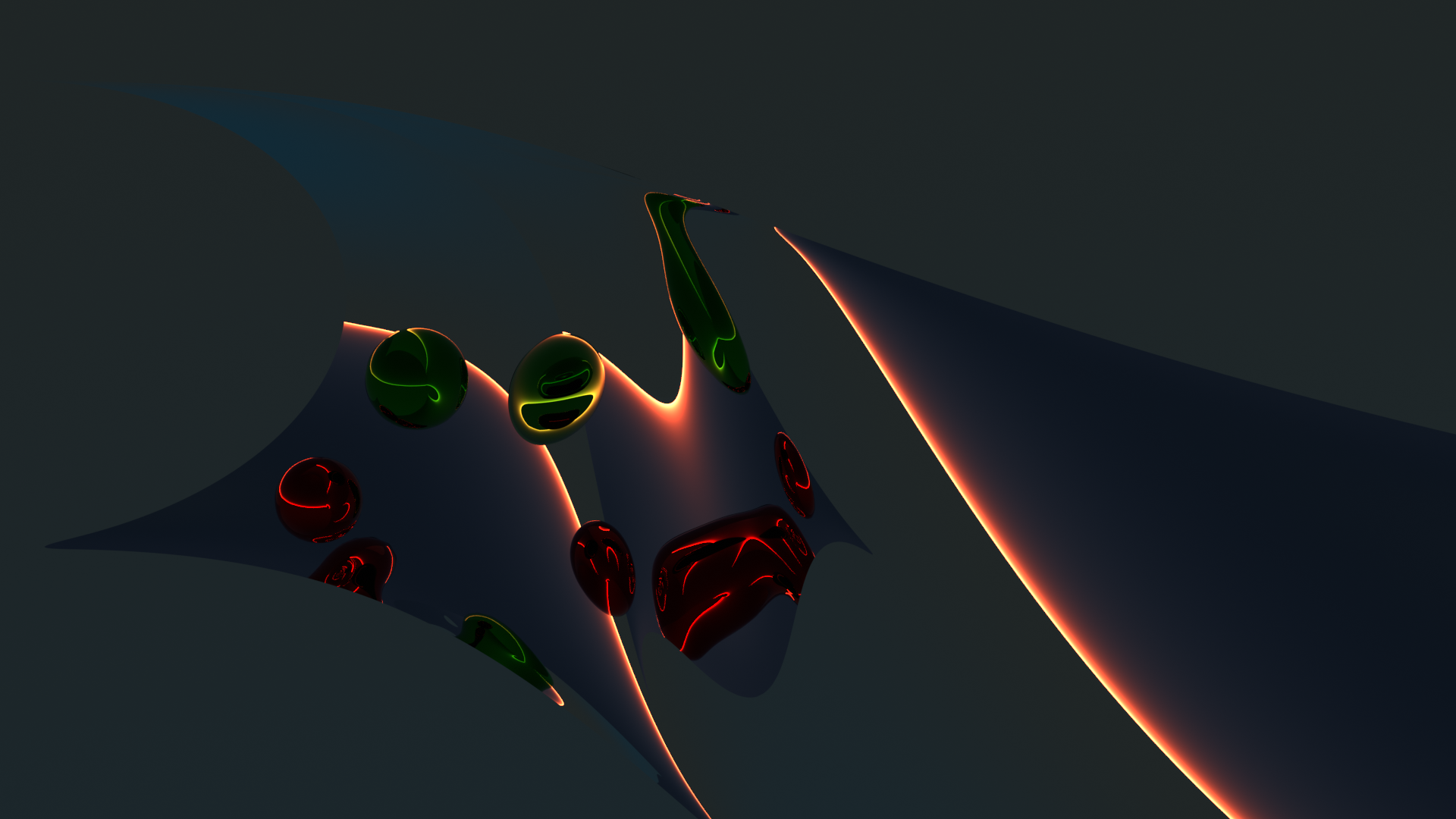
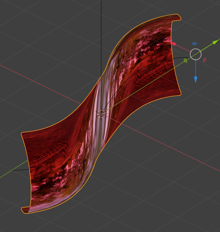
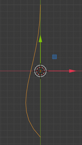
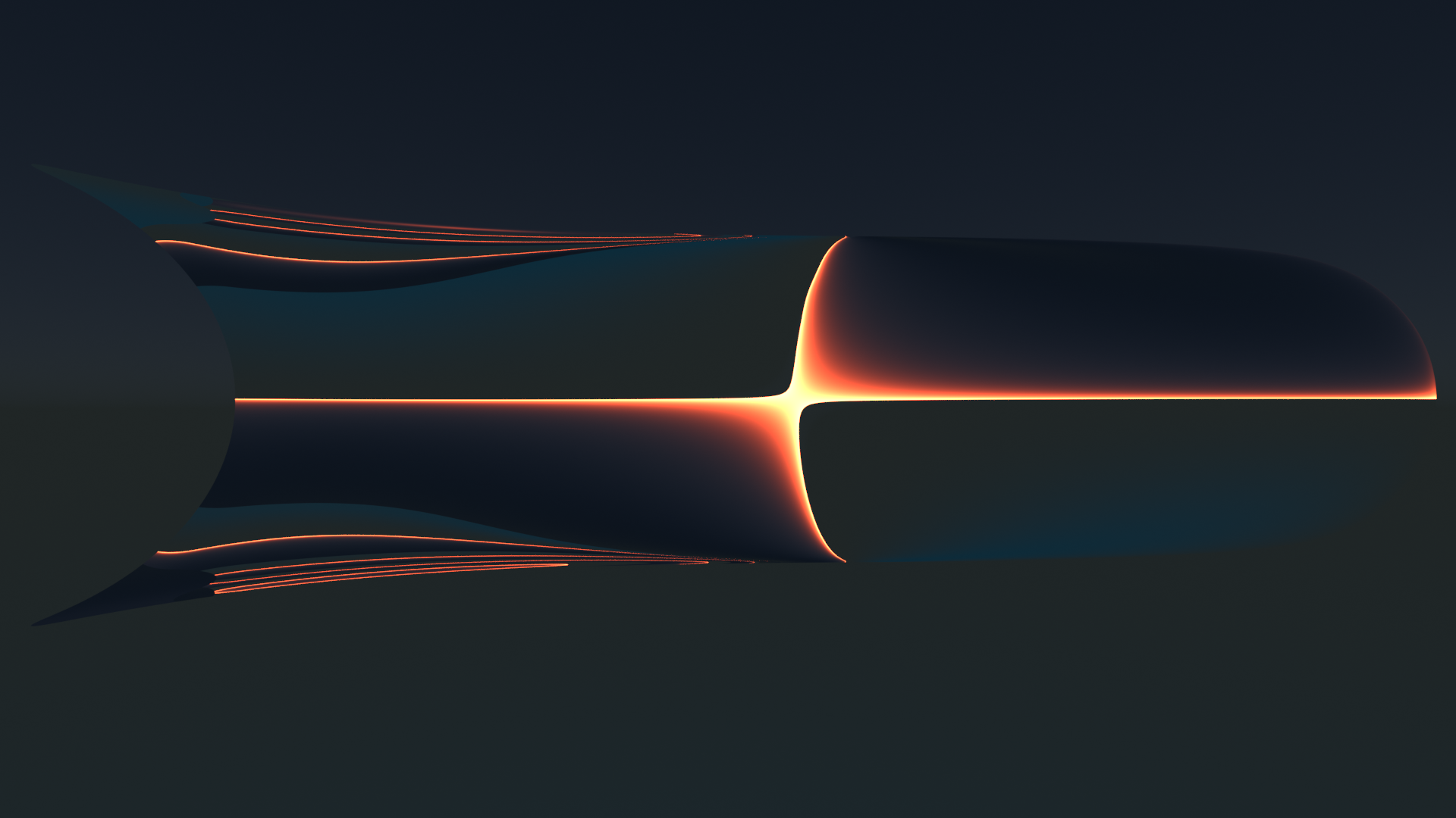
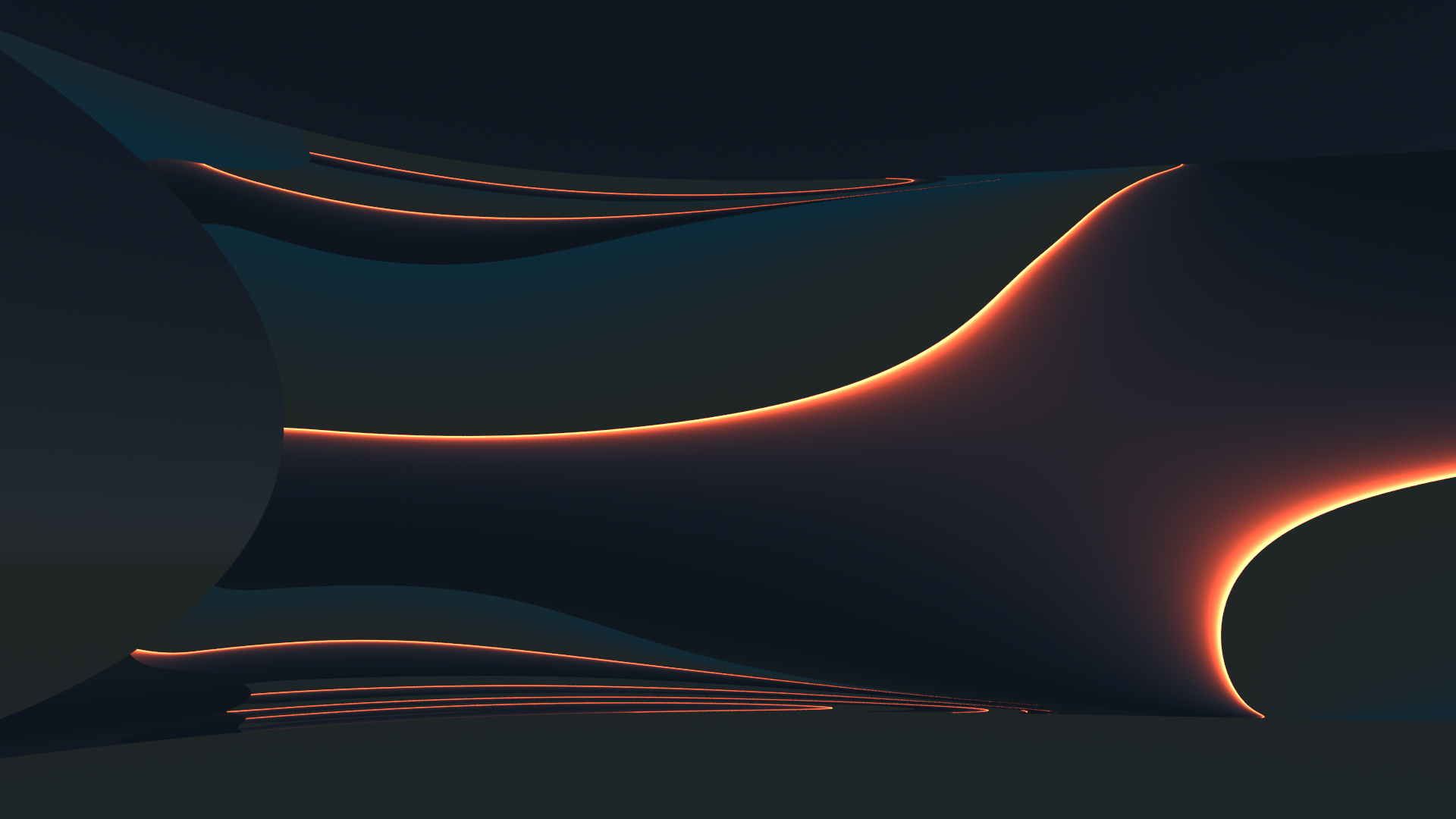
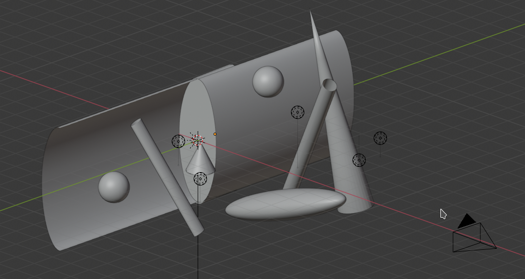
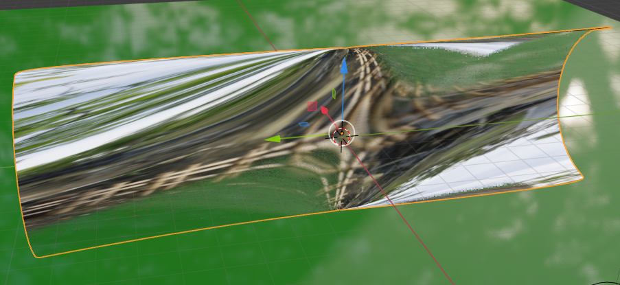
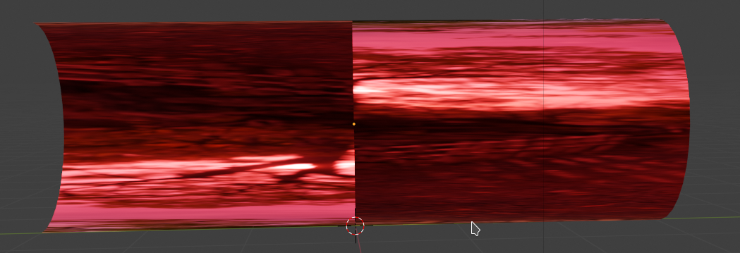
After having created such an object we can move and rotate it as we like. In the following images I mirrored it (2 rotations!). The concave curvature is now at the right side. Then I added a plane with some minimum texture with disturbances. Eventually, I added some objects and extended light sources, plus a change of the sun’s color to the red side of the spectrum. (Hint: When moving around spacious light sources relatively close to the object the reflections should not show any straight line disturbances. Its a way to test the smoothness of your surface created by the modifier.)

Yeah, one piece of metal with growing cylindrical concave and convex curvatures to the left and the right. We are getting closer to a reconstruction of the S-curve. And have a look at the nice deformations of the reflected images of a red cylinder, a green cone and a blue sphere, which I have placed relatively closely to the concave surface on the right side. Physics and Blender are fun! But all respect and tribute again to Anish Kapoor for his original idea!
In the next post
Blender – complexity inside spherical and concave cylindrical mirrors – III – a second step towards the S-curve
I have a look at an additional S-curvature in horizontal direction. Stay tuned ..