I continue with my series on a simple CNN used upon the MNIST dataset.
A simple CNN for the MNIST dataset – V – about the difference of activation patterns and features
A simple CNN for the MNIST dataset – IV – Visualizing the activation output of convolutional layers and maps
A simple CNN for the MNIST dataset – III – inclusion of a learning-rate scheduler, momentum and a L2-regularizer
A simple CNN for the MNIST datasets – II – building the CNN with Keras and a first test
A simple CNN for the MNIST datasets – I – CNN basics
In the last article I discussed the following points:
- The series of convolutional transformations, which a CNN applies to its input, eventually leads to abstract representations in low dimensional parameter spaces, called maps. In the case of our CNN we got 128 (3×3)-maps at the last convolutional layer. 3×3 indeed means a very low resolution.
- We saw that the transformations would NOT produce results on the eventual maps which could be interpreted in the sense of figurative elements of depicted numbers, such as straight lines, circles or bows. Instead, due to pooling layers, lines and curved line elements obviously experience a fast dissolution during propagation through the various Conv layers. Whilst the first Conv layer still gives fair representations of e.g. a “4”, line-like structures get already unclear at the second Conv layer and more or less disappear at the maps of the last convolutional layer.
- This does not mean that a map on a deep convolutional layer does not react to some specific pattern within the pixel data of an input image. We called such patterns OIPs in last article and we were careful to describe them as geometrical correlations of pixels – and not conceptual entities. The sequence of convolutions which makes up a map on a deep convolutional layer corresponds to a specific combination of filters applied to the image data. This led us to the the theoretical idea that a map may indeed select a specific OIP in an input image and indicate the existence of such a OIP pattern by some activation pattern of the “neurons” within the map. However, we have no clue at the moment what such OIPs may look like and whether they correspond to conceptual entities which other authors usually call “features”.
- We saw that the common elements of the maps of multiple images of a handwritten “4” correspond to point-like activations within specific low dimensional maps on the output side of the last convolutional layer.
- The activations seem to form abstract patterns across the maps of the last convolutional layer. These patterns, which we called FCPs, seem to support classification decisions, which the MLP-part of the CNN has to make.
So, at our present level of the analysis of a CNN, we cannot talk in a well founded way about “features” in the sense of conceptual entities. We got, however, the impression that eventual abstractions of some patterns which are present in MNIST images of different digits lead to FCP patterns across maps which allow for a classification of the images (with respect to the represented digits). We identified at least some common elements across the eventual maps of 3 different images of handwritten “4”s.
But it is really this simple? Can we by just looking for visible patterns in the activation output of the last convolutional layer already discriminate between different digits?
In this article I want to show that this is NOT the case. To demonstrate this we shall look at the image of a “4” which could also be almost classified to represent a “9”. We shall see
- that the detection of clear unique patterns becomes really difficult when we look at the representations of “4”s which almost resemble a “9” – at least from a human point of view;
- that directly visible patterns at the last convolutional layer may not contain sufficiently clear information for a classification;
- that the MLP part of our CNN nevertheless detects patterns after a linear transformation – i.e. after a linear combination of the outputs of the last Conv layer – which are not directly evident for human eyes. These “hidden” patterns do, however, allow for a rather solid classification.
What have “4”s in common after three convolutional transformations?
As in the last article I took three clear “4” images
![]()
![]()
![]()
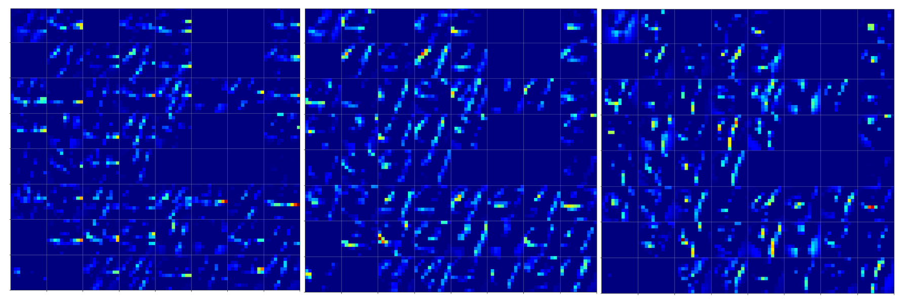
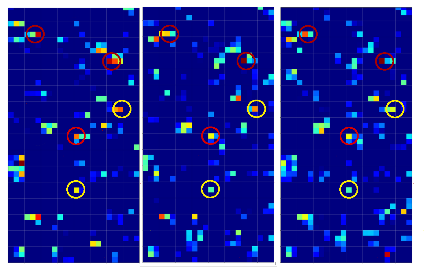
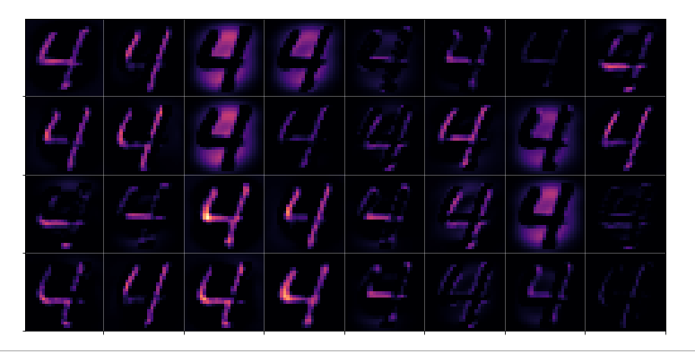
and compared the activation output after three convolutional transformations – i.e. at the output side of the last Conv layer which we named “Conv2D_3”:
![]()
The red circles indicate common points in the resulting 128 maps which we do not find in representations of three clear “9”s (see below). The yellow circles indicate common patterns which, however, appear in some representations of a “9”.
What have “9”s in common after three convolutional transformations?
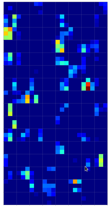
Now let us look at the same for three clear “9”s:
![]()
![]()
![]()
A comparison gives the following common features of “9”s on the third Conv2D layer:
![]()
We again get the impression that enough unique features seem to exist on the maps for “4”s and “9”s, respectively, to distinguish between images of these numbers. But is it really so simple?
Intermezzo: Some useful steps to reproduce results
You certainly do not want to perform a training all the time when you want to analyze predictions at certain layers for some selected MNIST images. And you may also need the same “X_train”, “X_test” sets to identify one and the same image by a defined number. Remember: In the Python code which I presented in a previous article for the setup for the data samples no unique number would be given due to initial shuffling.
Thus, you may need to perform a training run and then save the model as well as your X_train, y_train and X_test, y_test datasets. Note that we have transformed the data already in a reasonable tensor form which Keras expects. We also had already used one-hot-labels. The transformed sets were called “train_imgs”, “test_imgs”, “train_labels”, “test_labels”, “y_train”, “y_test”
The following code saves the model (here “cnn”) at the end of a training and loads it again:
# save a full model
cnn.save('cnn.h5')

#load a full model
cnnx = models.load_model('cnn.h5')
On a Linux system the default path is typically that one where you keep your Jupyter notebooks.
The following statements save the sets of tensor-like image data in Numpy compatible data (binary) structures:
# Save the data

from numpy import save
save('train_imgs.npy', train_imgs)
save('test_imgs.npy', test_imgs)
save('train_labels.npy', train_labels)
save('test_labels.npy', test_labels)
save('y_train.npy', y_train)
save('y_test.npy', y_test)
We reload the data by
# Load train, test image data (in tensor form)

from numpy import load
train_imgs   = load('train_imgs.npy')
test_imgs    = load('test_imgs.npy')
train_labels = load('train_labels.npy')
test_labels  = load('test_labels.npy')
y_train      = load('y_train.npy')
y_test       = load('y_test.npy')
Be careful to save only once – and not to set up and save your training and test data again in a pure analysis session! I recommend to use different notebooks for training and later analysis. If you put all your code in just one notebook you may accidentally run Jupyter cells again, which you do not want to run during analysis sessions.
What happens for unclear representations/images of a “4”?
When we trained a pure MLP on the MNIST dataset we had a look at the confusion matrix:
A simple Python program for an ANN to cover the MNIST dataset – XI – confusion matrix.
We saw that the MLP e.g. confused “5”s with “9s”, “9”s with “4”s, “2”s with “7”s, “8”s with “5”s – and vice versa. We got the highest confusion numbers for the misjudgement of badly written “4”s and “9”s.
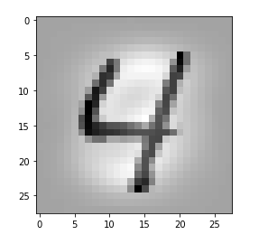
Let us look at a regular 4 and two “4”s which with some good will could also be interpreted as representations of a “9”; the first one has a closed upper area – and there are indeed some representations of “9”s in the MNIST dataset which look similar. The second “4” in my view is even closer to a “9”:
![]()
![]()
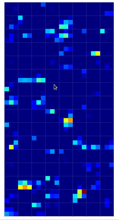
Now, if we wanted to look out for the previously discussed “unique” features of “4”s and “9s” we would get a bit lost:
![]()
The first image is for a clear “4”. The last two are the abstractions for our two newly chosen unclear “4”s in the order given above.
You see: Many of our seemingly “unique features” for a “4” on the third Conv-level are no longer or not fully present for our second “4”; so we would be rather insecure if we had to judge the abstraction as a viable pattern for a “4”. We would expect that this “human” uncertainty also shows up in a probability distribution at the output layer of our CNN.
But, our CNN (including its MLP-part) has no doubt about the classification of the last sample as a “4”. We just look at the prediction output of our model:
# Predict for a single image
# ****************************
num_img = 1302
ay_sgl_img = test_imgs[num_img:num_img+1]
print(ay_sgl_img.shape)
# load last cell for the next statement to work
#prob = cnn_pred.predict_proba(ay_sgl_img, batch_size=1)
#print(prob)
prob1 = cnn_pred.predict(ay_sgl_img, batch_size=1)
print(prob1)

[[3.61540742e-07 1.04205284e-07 1.69877489e-06 1.15337198e-08
  9.35641170e-01 3.53500056e-08 1.29525617e-07 2.28584581e-03
  2.59062881e-06 6.20680153e-02]]
93.5% probability for a “4”! A very clear discrimination! How can that be, given the – at first sight – seemingly unclear pattern situation at the third activation layer for our strange 4?
The MLP-part of the CNN “sees” things we humans do not see directly
We shall not forget that the MLP-part of the CNN plays an important role in our game. It reduces the information of the last 128 maps (3x3x128 = 1152) values down to 100 node values with the help of 115200 distinguished weights for related connections. This means there is a lot of fine-tuned information extraction and information compactification going on at the border of the CNN’s MLP part – a transformation step which is too complex to grasp directly.
It is the transformation of all the 128x3x3-map-data into all 100 nodes via a linear combination which makes things difficult to understand. 115200 optimized weights leave enough degrees of freedom to detect combined patterns in the activation data which are more complex and less obvious than the point-like structures we encircled in the images of the maps.
So, it is interesting to visualize and see how the MLP part of our CNN reacts to the activations of the last convolutional layers. Maybe we find some more intriguing patterns there, which discriminate “4”s from “9”s and explain the rather clear probability evaluation.
Visualization of the output of the dense layers of the CNN’s MLP-part
We need to modify some parts of our code for creating images of the activation outputs of convolutional layers to be able to produce equally reasonable images for the output of the dense MLP layers, too. These modifications are simple. We distinguish between the types of layers by their names: When the name contains “dense” we execute a slightly different code. The changes affect just the function “img_grid_of_layer_activation()” previously discussed as the contents of a Jupyter “cell 9“:
# Function to plot the activations of a layer
# --------------------------
-----------------
# Adaption of a method originally designed by F.Chollet

def img_grid_of_layer_activation(d_img_sets, model_fname='cnn.h5', layer_name='', img_set="test_imgs", num_img=8,
                                 scale_img_vals=False):
    '''
    Input parameter:
    -----------------
    d_img_sets: dictionary with available img_sets, which contain img tensors (presently: train_imgs, test_imgs)
    model_fname: Name of the file containing the models data
    layer_name: name of the layer for which we plot the activation; the name must be known to the Keras model (string)
    image_set: The set of images we pick a specific image from (string)
    num_img: The sample number of the image in the chosen set (integer)
    scale_img_vals: False: Do NOT scale (standardize) and clip (!) the pixel values. True: Standardize the values. (Boolean)

    Hints:
    -----------------
    We assume quadratic images - in case of dense layers we assume a size of 1
    '''

    # Load a model
    cnnx = models.load_model(model_fname)

    # get the output of a certain named layer - this includes all maps
    # https://keras.io/getting_started/faq/#how-can-i-obtain-the-output-of-an-intermediate-layer-feature-extraction
    cnnx_layer_output = cnnx.get_layer(layer_name).output

    # build a new model for input "cnnx.input" and output "output_of_layer"
    # ~~~~~~~~~~~~~~~~~
    # Keras knows the required connections and intermediat layers from its tensorflow graphs - otherwise we get an error
    # The new model can make predictions for a suitable input in the required tensor form
    mod_lay = models.Model(inputs=cnnx.input, outputs=cnnx_layer_output)

    # Pick the input image from a set of respective tensors
    if img_set not in d_img_sets:
        print("img set " + img_set + " is not known!")
        sys.exit()
    # slicing to get te right tensor
    ay_img = d_img_sets[img_set][num_img:(num_img+1)]

    # Use the tensor data as input for a prediction of model "mod_lay"
    lay_activation = mod_lay.predict(ay_img)
    print("shape of layer " + layer_name + " : ", lay_activation.shape )

    # number of maps of the selected layer
    n_maps   = lay_activation.shape[-1]
    print("n_maps = ", n_maps)

    # size of an image - we assume quadratic images
    # in the case  of "dense" layers we assume that the img size is just 1 (1 node)
    if "dense" in layer_name:
        img_size = 1
    else:
        img_size = lay_activation.shape[1]
    print("img_size = ", img_size)

    # Only for testing: plot an image for a selected
    # map_nr = 1
    #plt.matshow(lay_activation[0,:,:,map_nr], cmap='viridis')

    # We work with a grid of images for all maps
    # ~~~~~~~~~~~~~~~----------------------------
    # the grid is build top-down (!) with num_cols and num_rows
    # dimensions for the grid
    num_imgs_per_row = 8
    num_cols = num_imgs_per_row
    num_rows = n_maps // num_imgs_per_row
    #print("img_size = ", img_size, " num_cols = ", num_cols, " num_rows = ", num_rows)

    # grid
    dim_hor = num_imgs_per_row * img_size
    dim_ver = num_rows * img_size
    img_grid = np.zeros( (dim_ver, dim_hor) )   # horizontal, vertical matrix
    print("shape of img grid = ", img_grid.shape)

    # double loop to fill the grid
    n = 0
    for row in range(num_rows):
        for col in range(num_cols):
            n += 1
            #print("n = ", n, "row = ", row, " col = ", col)
            # in case of a dense layer the shape of the tensor like output
            # is different in comparison to Conv2D layers
            if "dense" in layer_name:
                present_img = lay_activation[ :, row*num_imgs_per_row + col]
            else:

   present_img = lay_activation[0, :, :, row*num_imgs_per_row + col]

            # standardization and clipping of the img data
            if scale_img_vals:
                present_img -= present_img.mean()
                if present_img.std() != 0.0: # standard deviation
                    present_img /= present_img.std()
                    #present_img /= (present_img.std() +1.e-8)
                    present_img *= 64
                    present_img += 128
                present_img = np.clip(present_img, 0, 255).astype('uint8') # limit values to 255

            # place the img-data at the right space and position in the grid
            # ~~~~~~~~~~~~~~~~~~~~~~~~~~~~~~~~~~~~~~~~~~~~~~~~~~~~~~~~~~~~~~
            # the following is only used if we had reversed vertical direction by accident
            #img_grid[row*img_size:(row+1)*(img_size), col*img_size:(col+1)*(img_size)] = np.flip(present_img, 0)
            img_grid[row*img_size:(row+1)*(img_size), col*img_size:(col+1)*(img_size)] = present_img

    return img_grid, img_size, dim_hor, dim_ver
You certainly detect the two small changes in comparison to the code for Jupyter cell 9 of the article
A simple CNN for the MNIST dataset – IV – Visualizing the output of convolutional layers and maps.
However, there remains one open question: We were too lazy in the coding discussed in previous articles to create our own names names for the dense layers. This is, however, no major problem: Keras creates its own names – if we do not define our own layer names when constructing a CNN model. Where do we get these default names from? Well, from the model’s summary:
cnn_pred.summary()

Model: "sequential_7"
_________________________________________________________________
Layer (type)                 Output Shape              Param #
=================================================================
Conv2D_1 (Conv2D)            (None, 26, 26, 32)        320
_________________________________________________________________
Max_Pool_1 (MaxPooling2D)    (None, 13, 13, 32)        0
_________________________________________________________________
Conv2D_2 (Conv2D)            (None, 11, 11, 64)        18496
_________________________________________________________________
Max_Pool_2 (MaxPooling2D)    (None, 5, 5, 64)          0
_________________________________________________________________
Conv2D_3 (Conv2D)            (None, 3, 3, 128)         73856
_________________________________________________________________
flatten_7 (Flatten)          (None, 1152)              0
_________________________________________________________________
dense_14 (Dense)             (None, 100)               115300
_________________________________________________________________
dense_15 (Dense)             (None, 10)                1010
=================================================================
Total params: 208,982
Trainable params: 208,982
Non-trainable params: 0
_________________________________________________________________
Our first MLP layer with 100 nodes obviously got the name “dense_14”.
With our modification and the given name we can now call Jupyter “cell 10” as before:
# Plot the img grid of a layers activation
# ~~~~~~~~~~~~~~~~~~~~~~~~~~~~~~~~~~~~~~~~~

# global dict for the image sets
d_img_sets= {'train_imgs':train_imgs, 'test_imgs':test_imgs}

# layer - pick one of the names which you defined for your model
layer_name = "dense_14"

# choose a image_set and an img number
img_
set = "test_imgs"

# clear 4
num_img = 1816

#unclear 4
#num_img = 1270
#num_img = 1302

#clear 9
#num_img = 1249
#num_img = 1410
#num_img = 1858


# Two figures
# -----------
fig1 = plt.figure(1, figsize=(5,5))  # figure for the input img
fig2 = plt.figure(2)  # figure for the activation outputs of th emaps

fig1 = plt.figure( figsize=(5,5) )
ay_img = test_imgs[num_img:num_img+1]
#plt.imshow(ay_img[0,:,:,0], cmap=plt.cm.binary)
plt.imshow(ay_img[0,:,:,0], cmap=plt.cm.jet)


# getting the img grid
img_grid, img_size, dim_hor, dim_ver = img_grid_of_layer_activation(
                                        d_img_sets, model_fname='cnn.h5', layer_name=layer_name,
                                        img_set=img_set, num_img=num_img,
                                        scale_img_vals=False)
# Define reasonable figure dimensions by scaling the grid-size
scale = 1.6 / (img_size)
fig2 = plt.figure( figsize=(scale * dim_hor, scale * dim_ver) )
#axes
ax = fig2.gca()
ax.set_xlim(-0.5,dim_hor-1.0)
ax.set_ylim(dim_ver-1.0, -0.5)  # the grid is oriented top-down
#ax.set_ylim(-0,dim_ver-1.0) # normally wrong

# setting labels - tick positions and grid lines
ax.set_xticks(np.arange(img_size-0.5, dim_hor, img_size))
ax.set_yticks(np.arange(img_size-0.5, dim_ver, img_size))
ax.set_xticklabels([]) # no labels should be printed
ax.set_yticklabels([])

# preparing the grid
plt.grid(b=True, linestyle='-', linewidth='.5', color='#ddd', alpha=0.7)

# color-map
#cmap = 'viridis'
#cmap = 'inferno'
cmap = 'jet'
#cmap = 'magma'

plt.imshow(img_grid, aspect='auto', cmap=cmap)
In the output picture each node will be represented by a colored rectangle.
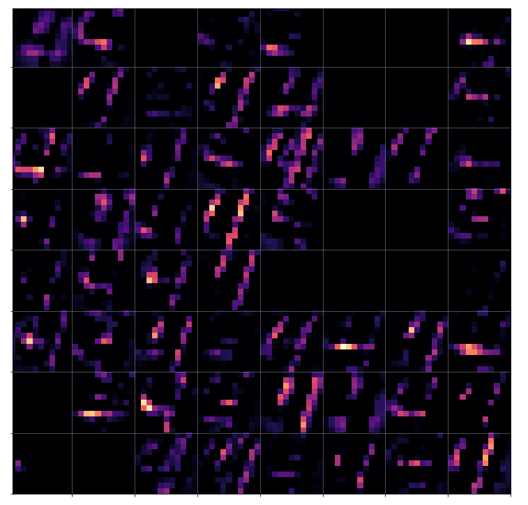
Visualization of the output for clear “4”s at the first dense MLP-layer
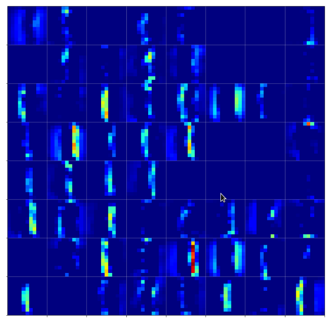
The following picture displays the activation values for three clear “4”s at the first dense MLP layer:
![]()
I encircled again some of the nodes which carry some seemingly “unique” information for representations of the digit “4”.
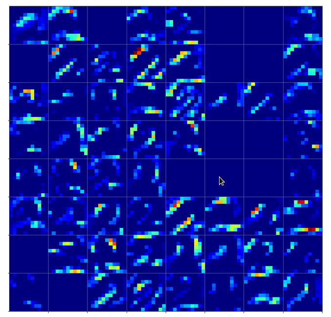
For clear “9”s we instead get:
![]()
Hey, there are some clear differences: Especially, the diagonal pattern (vertically a bit below the middle and horizontally a bit to the left) and the activation at the first node (upper left) seem to be typical for representations of a “9”.
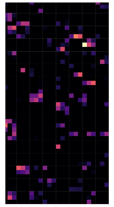
Our unclear “4” representations at the first MLP layer
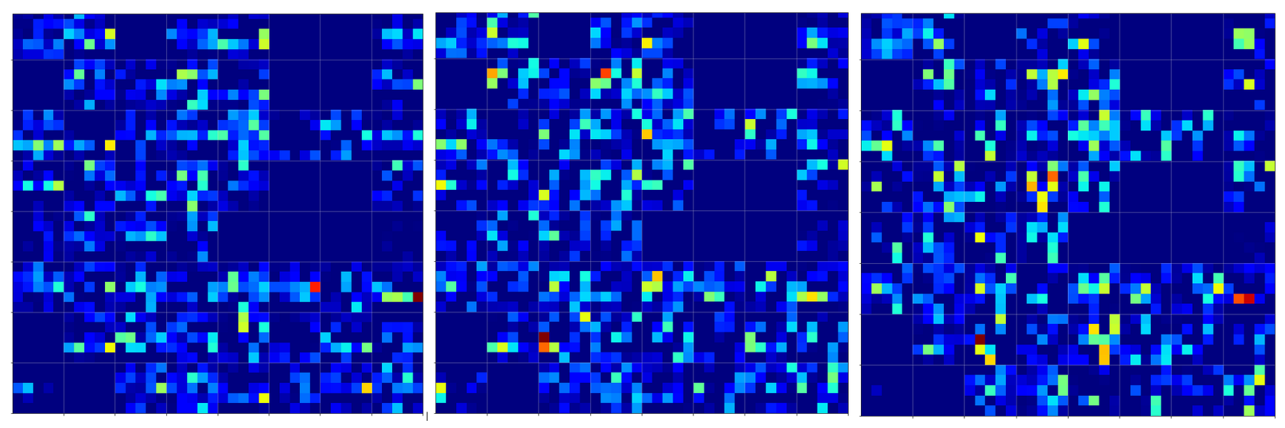
Now, what do we get for our two unclear “4”s?
![]()
I think that we would guess with confidence that our first image clearly corresponds to a “4”. With the second one we would be a bit more careful – but the lack of the mentioned diagonal structure with sufficiently high values (orange to yellow on the “jet”-colormap) would guide us to a “4”. Plus the presence of a relatively high value at a node present at the lower right which is nowhere in the “9” representations. Plus too small values at the upper left corner. Plus some other aspects – some nodes have a value where all the clear “9”s do not have anything.
We should not forget that there are more than 1000 weights again to emphasize some combinations and suppress others on the way to the output layer of the CNN’s MLP part.
Conclusion
Information which is still confusing at the last convolutional layer – at least from a human visual perspective – can be “clarified” by a combination of the information across all (128) maps. This is done by the MLP transformations (linear matrix plus non-linear activation function) which produce the output of the 1st dense layer.
Thus and of course, the dense layers of the MLP-part of a CNN play an important role in the classification process: The MLP may detect patterns in the the combined information of all available maps at the last convolutional layer which the human eye may have difficulties with.
In the sense of a critical review of the results of our last article we can probably say: NOT the individual points, which we marked in the images of the maps at the last convolutional layer, did the classification trick; it was the MLP analysis of the interplay of the information across all maps which in the end lead the CNN to an obviously correct classification.
Common features in calculated maps for MNIST images are nice, but without an analysis of a MLP across all maps they are not sufficient to solve the classification problem. So: Do not underestimate the MLP part of a CNN!
In the next article
I shall outline some required steps to visualize the patterns or structures within an input image which a specific CNN map reacts to. This will help us in the end to get a deeper understanding of the relation between FCPs and OIPs. I shall also present some first images of such OIP patterns or “features” which activate certain maps of our trained CNN.