In den ersten beiden Artikeln dieser Serie
KVM/qemu mit QXL – hohe Auflösungen und virtuelle Monitore im Gastsystem definieren und nutzen – I
KVM/qemu mit QXL – hohe Auflösungen und virtuelle Monitore im Gastsystem definieren und nutzen – II
hatte ich diskutiert, wie man das QXL-Device von Linux-Gastsystemen eines KVM/QEMU-Hypervisors für den performanten Umgang mit hohen Auflösungen vorbereitet.
Ich hatte zudem gezeigt, wie man mit Hilfe der Tools “xrandr” und “cvt” Auflösungen für Monitore unter einem X-Server einstellt.
Das funktioniert ganz unabhängig von Virtualisierungsaufgaben. So lassen sich u.U. auf Laptops und Workstations Auflösungen “erzwingen”, die trotz gegebener physikalischer Möglichkeiten der Grafikkarte und der angeschlossenen Monitoren nicht automatisch erkannt wurden. “cvt” nutzt man dabei zur Bestimmung der erforderlichen “modelines”.
“xrandr” funktioniert aber auch für X-Server virtualisierter Systeme – u.a. für Linux-Gastsysteme unter KVM/QEMU. Im Verlauf der letzten beiden Artikel hatten wir xrandr dann sowohl auf einem Linux-Virtualisierungs-Host wie auch in einem unter KVM/QEMU virtualisierten Linux-Gastsystem angewendet, um die jeweiligen KDE/Gnome-Desktops in angemessener Auflösung darzustellen.
Als praxisnahes Testobjekt musste dabei ein Laptop unter Opensuse Leap 42.2 herhalten, der mit KVM/QEMU ausgestattet war. Er beherbergte virtualisierte Gastsysteme unter “Debian 9 (Stretch)” und Kali2017. Ein relativ hochauflösender Monitor am HDMI-Ausgang (2560×1440) des Laptops konnte mit Hilfe von xrandr vollständig zur Darstellung der Gastsysteme genutzt werden, obwohl diese Auflösung vom Host nicht erkannt und nicht automatisch unterstützt wurde. Die grafische Darstellung des Gast-Desktops (Gnome/KDE) wurde dabei durch Spice-Clients auf dem Host und QXL-Devices in den virtuellen Maschinen ermöglicht.
Offene Fragen => Themen dieses Artikels
Eine Fragestellung an das bislang besprochene Szenario ist etwa, ob man mit hohen Auflösungen auch dann arbeiten kann, wenn die Spice-Clients auf einem anderen Linux-Host laufen als dem KVM-Virtualisierungshost selbst. Ich werde auf dieses Thema nur kurz und pauschal eingehen. Die Netzwerkkonfiguration von Spice und Libvirt werde ich bei Gelegenheit an anderer Stelle vertiefen.
Ergänzend stellte ein Leser zwischenzeitlich die Frage, ob man im Bedarfsfall eigentlich auch noch höhere Auflösungen für das Gastsystem vorgeben kann als die, die in einem physikalischen Monitor des Betrachter-Hosts unterstützt werden.
Für die Praxis ist zudem folgender Punkt wichtig:
Die bislang beschriebene manuelle Handhabung von QVT und xrandr zur Einstellung von Desktop-Auflösungen ist ziemlich unbequem. Das gilt im Besonderen für den Desktop des Gastsystems im Spice-Fenster. Wer hat schon Lust, jedesmal nach dem Starten eines Gastes “xrandr”-Befehle in ein Terminal-Fenster einzutippen? Das muss doch bequemer gehen! Wie also kann man die gewünschte Auflösung auf dem Betrachter-Host oder im virtualisierten Linux-Gastsystem persistent hinterlegen?
Noch idealer wäre freilich eine Skalierung der Auflösung des Gast-Desktops mit der Größe des Spice-Fensters auf dem Desktop des Anwenders. Lässt sich eine solche automatische Auflösungsanpassung unter Spice bewerkstelligen?
Der nachfolgende Artikel geht deshalb auf folgende Themen ein:
- Auflösungen und Vertikalfrequenzen für den Desktop des KVM-Gast, die physikalisch am Host des Betrachters nicht unterstützt
werden.
- Persistenz der xrandr-Einstellungen für den Gast-Desktop und den dortigen Display-Manager (bzw. dessen Login-Fenster).
- Automatische (!) Auflösungsanpassung des Gast-Desktops an die Rahmengröße des Spice-Client-Fensters.
Zugriff auf virtualisierte Hosts über Netzwerke
Spice und libvirt sind netzwerkfähig! Siehe hierzu etwa http://www.linux-magazin.de/Ausgaben/2012/10/Spice. Das, was wir in den letzten beiden Artikeln bewerkstelligt haben, hätten wir demnach auch erreichen können, wenn wir xrandr nicht auf dem Virtualisierungshost selbst, sondern auf einem beliebigen Remote-Host zur Darstellung des Gast-Desktops in Spice-Fenstern eingesetzt hätten.
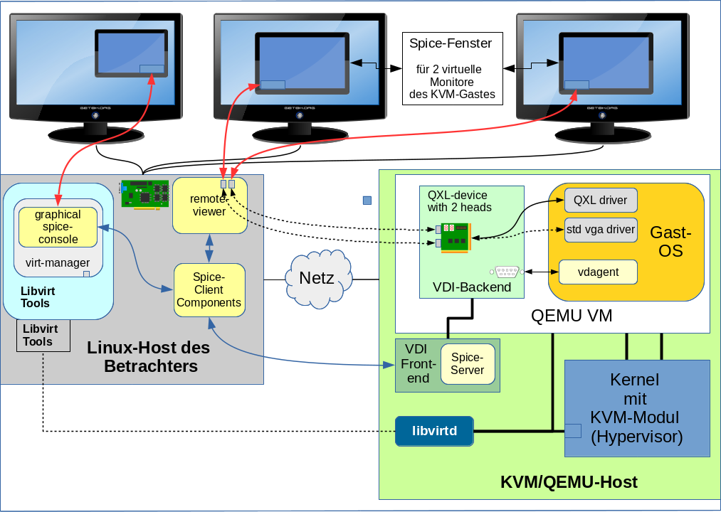
In den nachfolgenden Artikeln unterscheiden wir daher etwas genauer als bisher den “Linux-KVM-Host” vom “Host des Betrachters“. Letzteres liefert dem Anwender den “Desktop des Betrachters“, den wir vom “Desktop des virtualisierten Gastsystems” abgrenzen:
Auf dem “Desktop des Betrachters” werden Spice-Client-Fenster aufgerufen, über die der Anwender den Desktop des KVM-Gast-Systems betrachtet. Der “Linux-Host des Betrachters” kann also der KVM-Virtualisierungshost sein, muss es aber nicht. Die physikalisch mögliche Trennung zwischen dem Host, der den “Desktop des Betrachters” anzeigt, vom Linux-Host, auf dem ein Hypervisor das virtualisierte Gastsystem unterstützt, kommt in folgender Skizze zum Ausdruck:
Der Einsatz von Libvirt und Spice über ein Netzwerk erfordert allerdings besondere System-Einstellungen. Ich werde erst in einem späteren Artikel zurückkommen. Die weiteren Ausführungen in diesem Artikel sind im Moment daher vor allem für Anwender interessant, die virtualisierte Systeme unter KVM auf ihrer lokalen Linux-Workstation betreiben. Leser, die unbedingt jetzt schon remote arbeiten wollen oder müssen, seien darauf hingewiesen, dass X2GO nach wie vor eine sehr performante Alternative zu Spice darstellt, die SSH nutzt, einfach zu installieren ist und headless, d.h. ganz ohne QXL, funktioniert.
Auflösungen und Vertikalfrequenzen des Gastdesktops jenseits der Möglichkeiten eines (einzelnen) physikalischen Monitors
Aufmerksame Leser haben am Ende des letzten Artikels sicherlich festgestellt, dass die in den virt-manager integrierte grafische Spice-Konsole Scrollbalken anbietet, wenn die Auflösung des darzustellenden Gast-Desktops die Rahmengröße des Spice-Fensters übersteigt. Das führt zu folgenden Fragen:
Kann man für den Desktop des Gastsystems auch Auflösungen vorgeben, die die physikalischen Grenzen eines am Betrachter-Host angeschlossenen Monitors übersteigen?
Antwort: Ja, man kann für den Gast durchaus höhere Auflösungen vorgeben als die, die ein physikalischer Monitor unterstützt. Das führt logischerweise zu einer pixelmäßig nicht schärfer werdenden Vergrößerung der Desktop-Fläche des Gastes. Man muss dann eben im Spice-Fenster scrollen, wenn man das Spice-Fenster nicht über die Größe des fraglichen physikalischen Monitors ausdehnen kann.
Haben höhere Gast-Auflösungen als die eines physikalischen Monitors überhaupt einen Sinn?
Antwort: Ja – nämlich dann, wenn man am Linux-Host, von dem aus man den Gast-Desktop betrachtet, mehrere Monitore per “xinerama” zu einem von der Pixelfläche her zusammenhängenden Monitor gekoppelt hat!
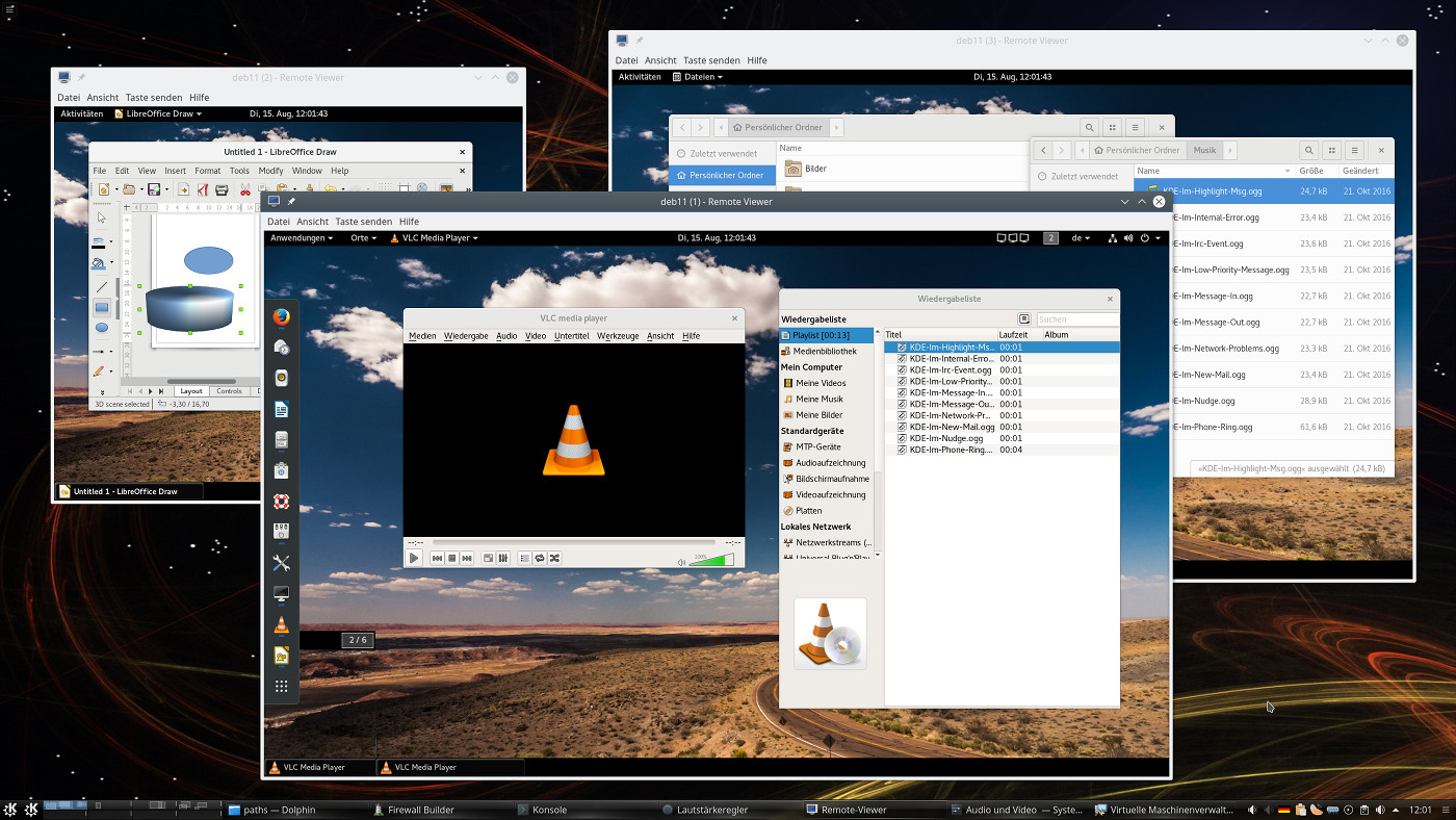
An einem von mir betreuten System hängen etwa drei Monitore mit je max. 2560×1440 px Auflösung. Nachfolgend seht ihr ein Bild von einem testweise installierten Debian-Gast, für den mittels CVT und xrandr eine Auflösung von 5120×1080 Pixel eingestellt wurde. Das Spice-Fenster auf dieser Linux-Workstation erstreckt sich dann über 2 von 3 physikalischen Monitoren. Siehe die linke Seite der nachfolgenden Abbildung:
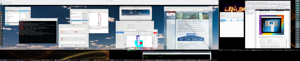
Von der grafischen Performance her ist das auf diesem System (Nvidia 960GTX) überhaupt kein Problem; der Gewinn für den Anwender besteht in komfortablem Platz zum Arbeiten auf dem Desktop des Gastsystems! In der Regel bedeutet das nicht mal eine Einschränkung für das Arbeiten mit dem Desktop des Betrachter-Hosts: Man kann unter KDE oder Gnome ja beispielsweise einfach auf eine weitere, alle drei Monitore überstreckende “Arbeitsfläche” des Betrachter-Desktops ausweichen.
U.a. ist es auch möglich, 4K-Auflösungen, also 4096 × 2160 Pixel, für den Desktop des virtualisierten Systems einzustellen. Man hat dann entweder physikalische Monitore am Betrachter-Host verfügbar, die 4K unterstützen, oder genügend Monitore mit geringerer Auflösung zusammengeschlossen – oder man muss, wie gesagt, eben scrollen. Für manche Grafik-Tests mag selbst Letzteres eine interessante Option sein.
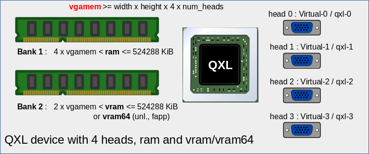
Gibt es Grenzen für die einstellbare QXL-Auflösung des virtualisierten Gast-Systems?
Antwort: Ja; momentan unterstützt das QXL-Device maximal 8192×8192 Pixel.
Geht man so hoch, muss man, wie bereits im ersten Artikel beschrieben, aber auch den Video-RAM des QXL-Devices anpassen und ggf. auf den Parameter “vram64” zurückgreifen!
Nachtrag 15.08.2017:
Nutzt man ein Memory/RAM der VM > 2048 MiB, so gibt es zusätzliche Einschränkungen für den maximalen ram-Wert des QXL-Devices. S. hierzu die inzwischen eingefügten Hinweise im ersten Artikel.
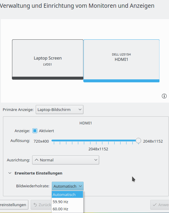
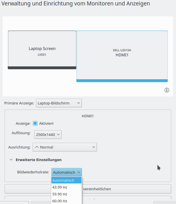
Funktionieren bei den Gastsystem-Einstellungen auch andere Vertikalfrequenzen als solche, die vom physikalischen Monitor unterstützt werden?
Antwort: Ja, auch das funktioniert!
Z.B. unterstützt der in den vorhergehenden Artikeln angesprochene Laptop die Auflösung 2560×1440 physikalisch nur mit 44Hz. Dennoch kann ich für den virtualisierten Gast-Desktop auch Modelines für eine Vertikalfrequenz von 60Hz oder 20Hz anfordern. Das macht in der finalen Darstellung auf dem Host des Betrachters nichts aus – die Grafik-Information wird ja lediglich in das dortige Spice-Fenster eingeblendet; die Abfrage von Änderungen am virtuellen Desktop erfolgt von Spice und QEMU (vermutlich) mit eigenen, intern definierten Frequenzen und wird entsprechend zwischen Spice-Server und -Client übertragen. Aber es schadet nicht, bei der Wahl der Vertikalfrequenz für die Video-Modes des Gastsystems einen vernünftigen Wert wie 60Hz oder 50HZ zu wählen.
Persistenz der Auflösungseinstellungen
Es gibt verschiedene Wege, per CVT gefundene Auflösungen und deren Modelines permanent in einem Linux-System zu hinterlegen und diese Modes beim Start einer graphischen Desktop-Sitzung direkt zu aktivieren. Der Erfolg des einen oder anderen Weges ist aber immer auch ein wenig distributions- und desktop-abhängig.
Ich konzentriere mich nachfolgend nur auf ein Debian-Gast-System mit Gnome 3 und gdm3 als Display Manager. Ich diskutiere dafür auch nur 2 mögliche Ansätze. Für KDE5 und SDDM gibt es allerdings ähnliche Lösungen ….
Warnhinweis:
Am Beispiel des bereits diskutierten Laptops sollte klargeworden sein, dass solche
Einstellungen ggf. sowohl im virtualisierten Gastsystem als auch auf dem Linux-Host, an dem die physikalischen Monitore hängen, dauerhaft hinterlegt werden müssen. Bzgl. der physikalisch wirksamen Einstellungen auf dem eBtrachter-Host ist allerdings Vorsicht geboten; man sollte seine Video-Modes und Frequenzen dort unbedingt im Rahmen der unterstützten Monitor- und Grafikartengrenzen wählen.
Variante 1 – rein lokale, userspezifische Lösung: Eine distributions- und desktop-neutrale Variante wäre etwa, die xrandr-Kommandos in einer Datei “~/.profile” für den Login-Vorgang oder (besser!) in einer Autostart-Datei für das Eröffnen der graphischen Desktop-Sitzung zu hinterlegen. Siehe hierzu etwa:
https://askubuntu.com/ questions/ 754231/ how-do-i-save-my-new-resolution-setting-with-xrandr
Der Nachteil dieses Ansatzes ist, dass der User bereits wissen muss, welche Auflösungen man für seinen Monitor per “xrandr” sinnvollerweise einstellen kann und sollte. Beim “.profile”-Ansatz kommt hinzu, dass sich das bei jedem Login auswirkt. Falsche Modes sind auf der physikalischen Host-Seite aber, wie gesagt, problematisch. Es wäre besser, die User nutzten nur vom Admin vordefinierte Auflösungen und dies mit den üblichen Desktop-Tools. Einen entsprechenden Ausweg bietet die nachfolgende Methode.
Variante 2 – zentrale und lokale Festlegungen:
Dieser Weg führt über 2 Schritte; er ist ebenfalls neutral gegenüber diversen Linux-Varianten. Bei diesem Weg wird globale Information mit user-spezifischen Setzungen kombiniert:
Unter Opensuse Leap ist ein zentrales Konfigurationsverzeichnis “/etc/X11/xorg.conf.d/” für X-Sitzungen bereits vorhanden. Man kann dieses Verzeichnis aber auch unter Debian-Systemen manuell anlegen. Dort hinterlegt man dann in einer Datei “10-monitor.conf” Folgendes:
Section "Monitor"
	Identifier "Virtual-0"
	Modeline "2560x1440_44.00"  222.75  2560 2720 2992 3424  1440 1443 1448 1479 -hsync +vsync
	Option "PreferredMode" "2560x1440_44.00"
EndSection

Section "Screen"
	Identifier "Screen0"
	Monitor "Virtual-0"
	DefaultDepth 24
	SubSection "Display"
		Modes "2560x1440_44.00"
	EndSubsection
EndSection
Diese Statements hinterlegen eine definierte Auflösung – hier 2560×1440 bei 44Hz – für unseren virtuellen Schirm “Virtual-0” permanent. Die Modline haben wir, wie in den letzten Artikeln beschrieben, mittels CVT gewonnen. (Die angegebene Werte für die Modline und die Auflösung sind vom Leser natürlich dem eigenen System und den eigenen Wünschen anzupassen.)
Die obigen Festlegungen bedeuten nun aber noch nicht, dass nach einem weiteren Login eine neue Gnome- oder KDE-Sitzung unter Debian bereits die hohe Auflösung produzieren würde. Die “PreferredMode” wird vielmehr ignoriert. Warum ist mir, ehrlich gesagt, nicht klar. Egal: Die Auflösung steht immerhin in den lokalen Konfigurationstools des jeweiligen Desktops zur Auswahl zur Verfügung. Damit kann der Anwender dann die lokalen Auflösungswerte in persistenter Weise festlegen:
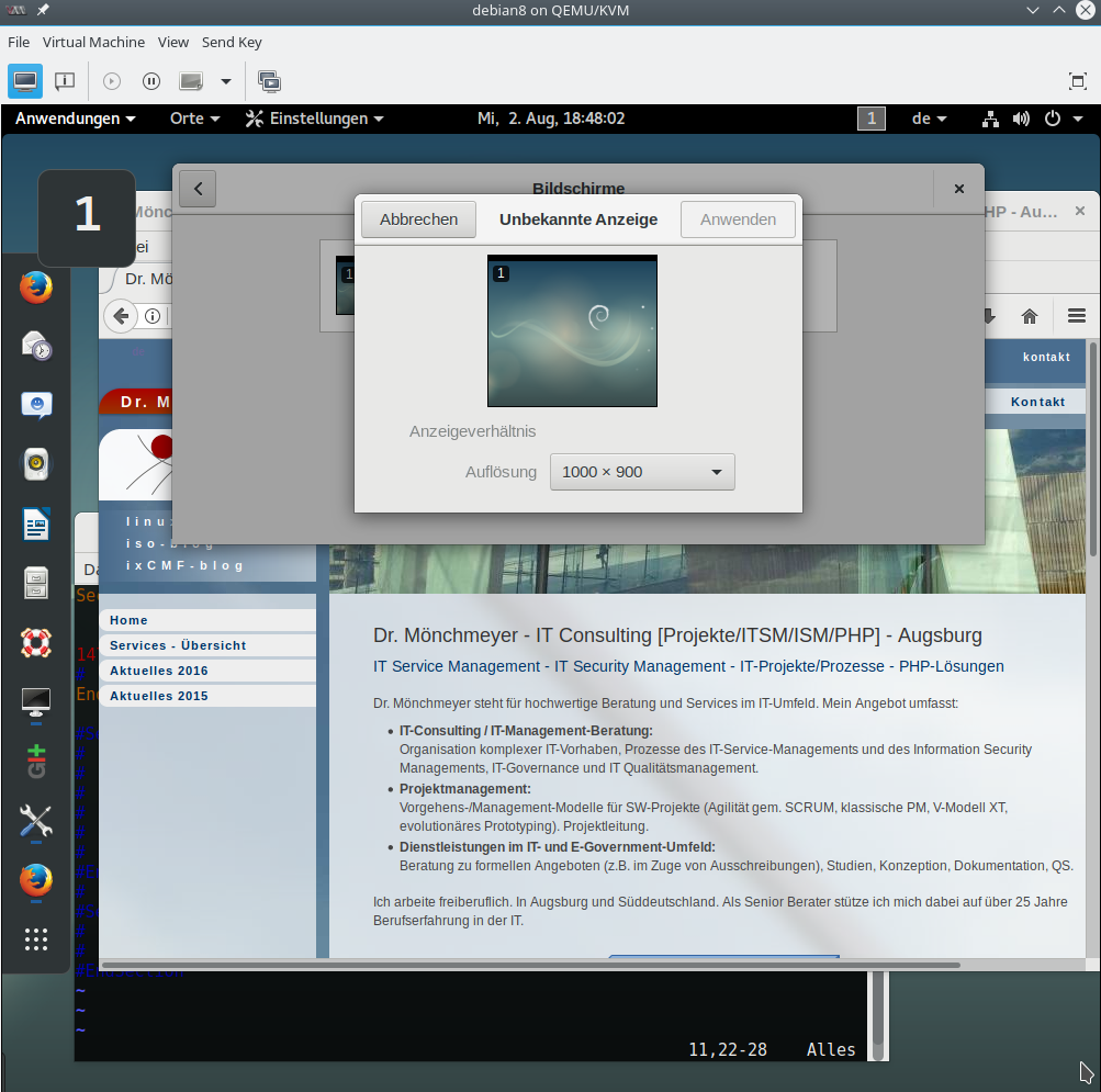
Unter “Gnome 3” rufen wir dazu im KVM-Gastsystem etwa das “gnome-control-center” auf:
myself@debian8:~$ gnome-control-center &
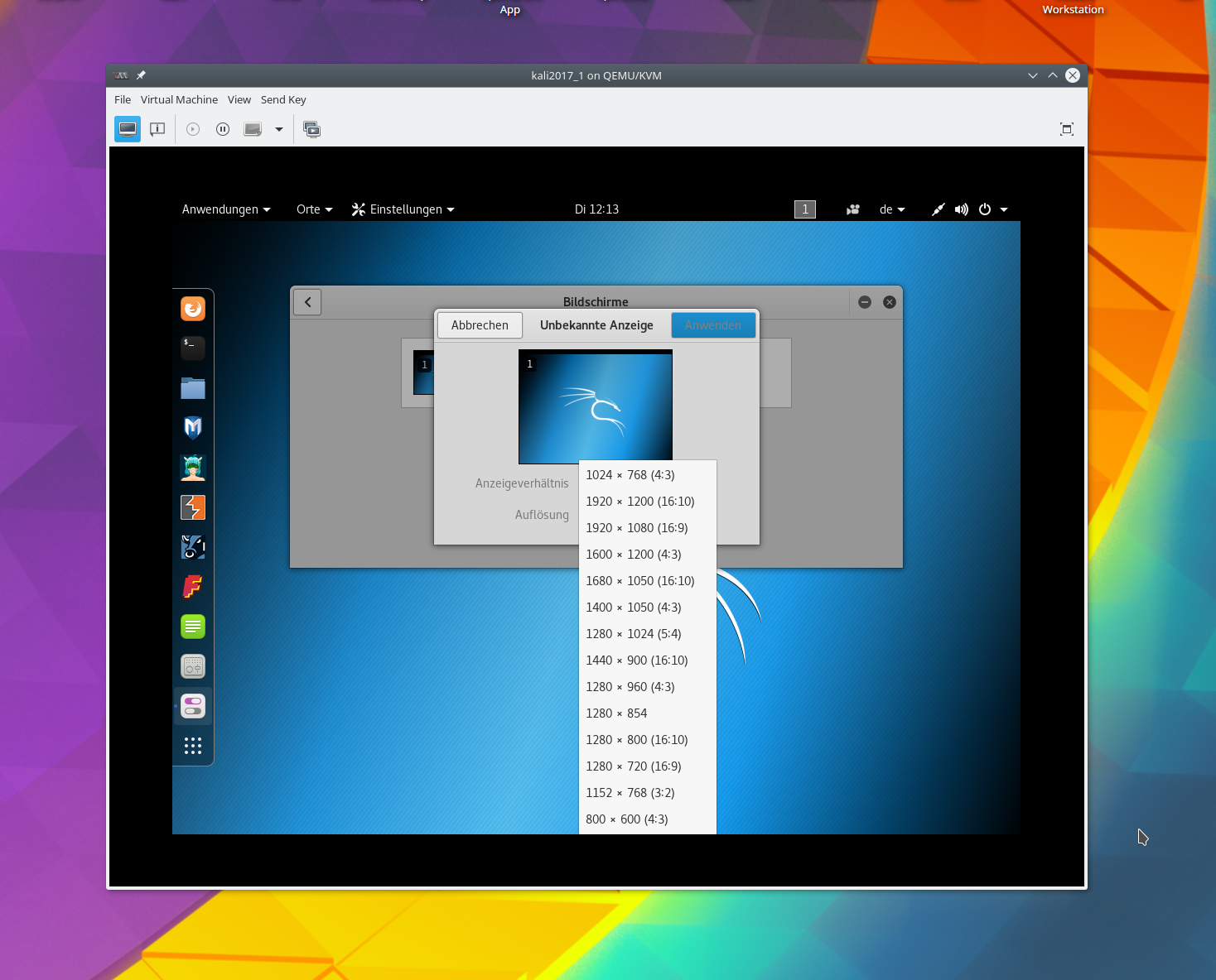
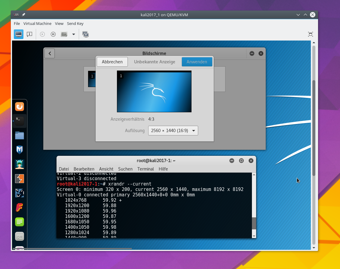
Dort wählen wir unter der Rubrik “Hardware” den Punkt “Bildschirme” und stellen die gewünschte Auflösung ein. Die Einstellung landet dann in einer Datei “~/.config/monitors.xml” – und ist X-Session-übergreifend verankert.
Im Falle von “KDE 5” wählen wir dagegen
myself@debian8:~$ systemsettings5 &
und dort dann den Punkt “Hardware >&
gt; Anzeige und Monitor”. Die dort getroffenen Einstellungen werden in einer Datei “~/.local/kscreen/” in einem JSON-ähnlichen Format gespeichert.
Diese 2-te Lösung hat den Vorteil, dass die maximale Auflösung systemweit vorgegeben wird. Der jeweilige User kann jedoch die von ihm gewünschte Einstellung wie gewohnt lokal hinterlegen und dafür die gewohnten Desktop-Tools einsetzen.
Persistenz der Auflösungseinstellungen für den “Display Manager” bzw. den Login-Schirm
Nachdem wir nun die Desktop-Sitzung unter Kontrolle haben, wäre es doch schön, auch das Login-Fenster des Display-Managers dauerhaft auf eine hohe Auflösung setzen zu können. Das geht am einfachsten für “gdm3”. 2 Varianten sind möglich:
Variante 1 – Globale Nutzung der Datei “monitors.xml”:
Die Festlegungen für den Gnome-Desktop wurden in einer Datei “~/.config/monitors.xml” festgehalten. Wir kopieren die “monitors.xml”-Datei nun als User “root” in das Verzeichnis “/var/lib/gdm3/.config/”:
root@debian8:~# cp /home/myself/.config/monitors.xml /var/lib/gdm3/.config/
Dort wird eine Konfigurationsdatei im XML-Format für den gdm3-Schirm ausgewertet. Unter Debian 8/9 hat sich hier allerdings ein Problem eingeschlichen:
gdm3 läuft dort bereits unter Wayland – und dieser X-Server ignoriert leider die getroffenen Einstellungen. Das lässt sich aber leicht beheben, indem man für gdm3 die Nutzung des klassischen X11-Servers erzwingt! In der Datei “/etc/gdm3/daemon.conf” muss dazu folgender Eintrag auskommentiert werden:
[daemon]
WaylandEnable=false
Danach wird dann beim nächsten gdm3-Start auch die “monitors.xml” akzeptiert – und die vorgeschlagene Auflösung übernommen. Leider ist es hier Benutzern ohne Root-Rechte nicht möglich, eigene Einstellungen zu treffen. Als Administrator sollte man hier natürlich zur HW passende Einstellungen wählen.
Links zum Thema “Ignoring monitors.xml in /var/lib/gdm3/.config/”
https://bugzilla.redhat.com/ show_bug.cgi? id=1184617
https://bugzilla.gnome.org/ show_bug.cgi? id=748098
In letzterem ist für Wayland auch ein Workaround beschrieben; ich habe das vorgeschlagene Vorgehen aber nicht getestet.
Variante 2: Nutzung von xrandr-Befehlen in Startup-Scripts des Display Managers
Man kann die “xrandr”-Befehle auch in den Startup-Scripts des jeweiligen Display Managers hinterlegen (xorg-Einstellungen werden leider grundsätzlich ignoriert). Für gdm3 also in der Datei “/etc/gdm3/Init/Default”. Dort kann man die xrandr-Anweisungen etwa am Dateiende anbringe. Siehe hierzu: https://wiki.ubuntu.com/X/ Config/ Resolution#Setting-xrandr-commands-in-kdm.2Fgdm_startup_scripts
Für mich ist das die präferierte Art, fixe Einstellungen für den Desktop-Display/Login-Manager vorzunehmen. Man muss sich allerdings für jeden der populären Manager (gdm3, ssdm, lightdm) kundig machen, in welcher Form Startup-Skripts eingebunden werden können. Leider gibt es dafür keinen Standard.
Nachtrag vom 02.03.2018:
Da “gdm3” im Moment unter aktuellen Debian- wie Kali-Installationen Probleme beim Shutdown macht (hängender Prozess, der von systemd nicht gestoppt werden kann), habe ich auch mal den simplen Login-Manager “lightdm” ausprobiert. Dort findet man Möglichkeiten zum Starten von Skripten in der Datei /etc/lightdm/lightdm.conf”. Siehe dort etwa die Option “display-setup-script”. Dort kann man auf bereits definierte Modes unter “/etc/X11/xorg.conf.d/10-monitor.conf” zurückgreifen – z.B. per “xrandr –output
Virtual-0 –mode 2560x1440_44.00”.
Automatische (!) Auflösungsanpassung des Gast-Desktops an die Größe des Spice-Client-Fensters
Die oben vorgeschlagenen Lösungen funktionieren zwar und mögen für den einen oder anderen Leser durchaus einen gangbaren Weg zur dauerhaften Nutzung hoher Auflösungen (genauer: großer Spice-Fenster-Abmessungen) von KVM/QEMU-Gastsystemen darstellen. Aber das ganze Procedere ist halt immer noch relativ arbeitsintensiv. Leute, die VMware nutzen, kennen dagegen die Möglichkeit, die Auflösung des Gastsystems direkt an die VMware-Fenstergröße anpassen zu lassen. Voraussetzung ist dort die Installation der sog. “VMware Tools” im Gastsystem. Gibt es etwas Korrespondierendes auch unter KVM/QXL/Spice ?
Antwort: Ja, aber …
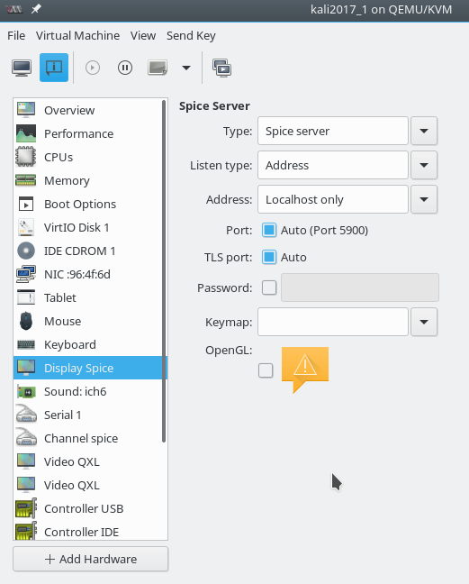
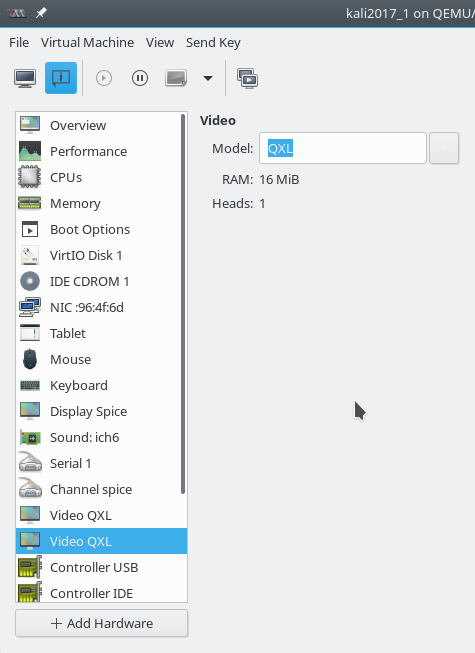
Eine Voraussetzung ist, dass der QXL-Treiber und der spice-vdagent im Gastsystem installiert und aktiv sind. Eine andere ist aktuell aber auch, dass der jeweilige grafische Desktop des KVM-Gastes (Gnome, KDE, …) mit diesem Duo und den von ihm bereitgestellten Informationen in sinnvoller Weise umgehen kann (s.u.).
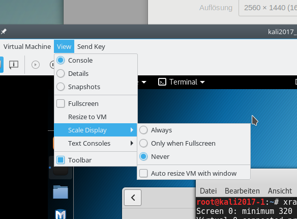
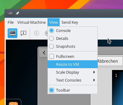
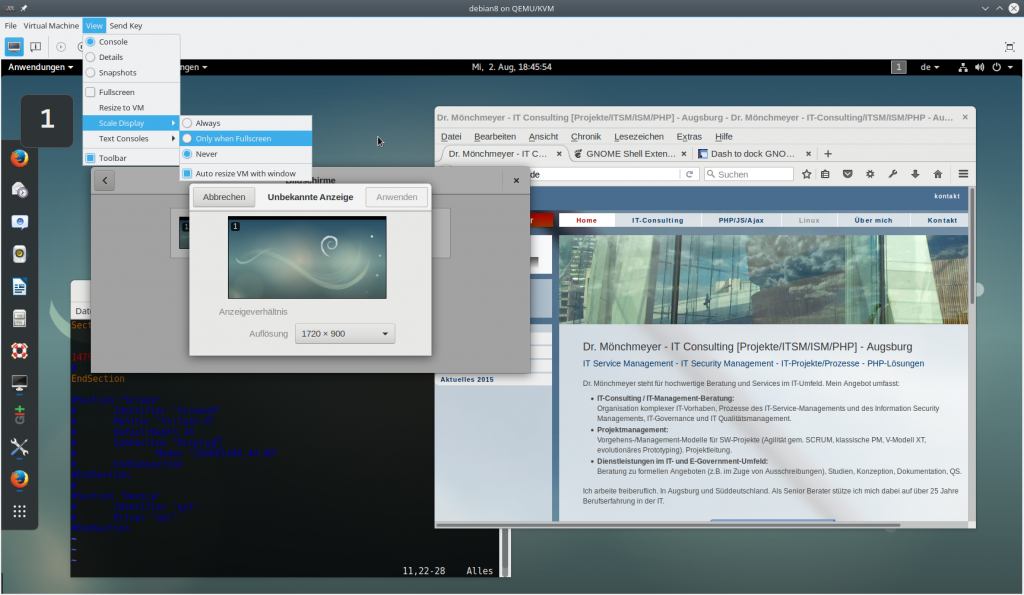
Die dynamische Desktop-Anpassung an die Spice-Fenstergröße kann durch KVM-Anwender über die Option
View >> Scale Display >> Auto resize VM with window
aktiviert werden. Die grafische Spice-Konsole (von virt-manager) bietet den entsprechenden Haupt-Menüpunkt in ihrer Menüleiste an.
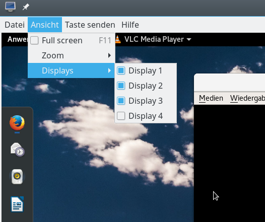
Nachtrag 02.03.2018:
Es gibt übrigens noch einen zweiten Spice-Client, den man über ein Terminal-Fenster starten kann – nämlich den sog. “Remote-Viewer” (siehe hierzu auch den nächsten Artikel dieser Serie). Je nach Versionsstand bietet der “Remote Viewer” entweder einen ähnlichen Menüpunkt an – oder aber der dargestellte Desktop des KVM-Gastes reagiert bei laufendem vdagent automatisch richtig, wenn im “Remote-Viewer” die Option “Ansicht (View) => Zoom => Normal Size” gewählt wird.
Nun verhält es sich leider so, dass sich das gewünschte Verhalten beim Aktivieren des Menüpunktes in einigen Fällen nicht unmittelbar einstellen mag.
Diesbzgl. sind als erstes 2 wichtige Punkte festzuhalten:
Hinweis 1: Die Funktionalität zur automatischen Auflösungsanpassung ist nicht völlig kompatibel mit den obigen Ansätzen zur Hinterlegung persistenter Auflösungseinstellungen! Im Besonderen muss man die Datei “/etc/X11/xorg.conf.d/10-monitor.conf” zunächst auf ein absolutes Minimum beschränken:
Section "Monitor"
	Identifier "Virtual-0"
	Modeline "2560x1440_44.00"  222.75  2560 2720 2992 3424  1440 1443 1448 1479 -hsync +vsync
EndSection
Oder man muss diese Datei gleich ganz entfernen.
Hinweis 2:
Manchmal passiert nichts, wenn man seine Spice-Screen-Größe schon verändert hat und erst dann die Option zur automatischen Anpassung an die Fenstergröße anklickt. Das irritiert den Anwender womöglich, der eine unmittelbare Reaktion erwartet. Die Informationen des Duos “vdagent/QXL-Treiber” zur Änderung der Größe des Spice-Client-Fensters werden offenbar aber erst dann erstmalig verarbeitet, wenn die Ausdehnung des Spice-Fensters tatsächlich durch den Nutzer geändert wird! Das Anklicken der Option im Menü allein ist also für eine erste Anpassung noch nicht ausreichend. Daher der Rat: Bitte testweise mit der Maus eine erste Größenänderung des Spice-Fensters vornehmen. Danach sollte der Desktop reagieren.
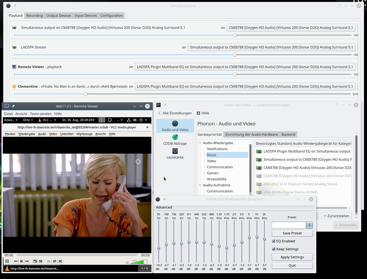
Ich zeige den Effekt in den nachfolgenden Bildern mal für ein “Debian 9”-Gast-System. Ich habe zwischen den Bildern dabei mit der Maus die Breite die Breite des Spice-Fensters auf dem KVM-Host von 1700px auf 1200px reduziert.
Aber auch das Beachten der oben genannten zwei Punkte ist im Moment in vielen Fällen nicht hinreichend. Zur Erläuterung muss man leider ein wenig ausholen. Früher war eine automatische Auflösungsanpassung u.a. Aufgabe des spice-vdagent. Im Moment gelten jedoch folgende Feststellungen:
- Politikwechsel: Red Hat hat aus (hoffentlich guten) Gründen die Politik bzgl. der Auflösungsanpassung geändert. Inzwischen nimmt nicht mehr der spice-vdagent die Auflösungsänderung vor, sondern überlässt dies dem aktuell laufenden Desktop (bzw. bzgl. des Login-Screens dem Desktop-Manager). Das Duo aus vdagent und QXL-Treiber übermittelt hierzu nur noch ein Signal samt der notwendigen Auflösungsinformationen an den aktuell laufenden Desktop (genauer an dessen kontrollierendes Programm) und überlässt ihm weitere Maßnahmen. Wobei die zugehörigen Programme vermutlich wiederum xrandr einsetzen. Für diesen Vorgang muss der QXL-Treiber (Kernelmodul!) aber auch geladen sein.
- Versionsabhängigkeiten: Eine automatische Auflösungsanpassung funktioniert aufgrund des Umbruchs bzgl. der Verantwortlichkeiten nicht mit allen Host- und Gast-Dristibutionen bzw. Programmständen von libvirt/spice bzw. QXL so wie erwartet.
Unter https://bugzilla.redhat.com/ show_bug.cgi? id=1290586 lesen wir entsprechend:
spice-vdagent used to be doing something like this, but this was racing with desktop environments keeping track of the current resolution/monitors/.., so we are now informing the desktop environment that a resolution change would be desirable, and let it handle it.
… It’s no longer going through spice-vdagent if you use the QXL KMS driver (although it needs spice-vdagent to be started iirc).
Dadurch ergeben sich aber neue Abhängigkeiten – denn wenn der QXL-Treiber und vdagent in einer aktuellen Version geladen sind, aber die jeweilige Desktop-Umgebung das Anliegen von QXL nicht unterstützt, geht halt nix. Mit den QXL-Anforderungen zur Auflösungsskalierung können nur neuere Versionen von Gnome und KDE vernünftig umgehen. Unter LXDE funktioniert im Moment leider überhaupt keine automatische Auflösungsanpassung mehr. Ein Beispiel für die etwas vertrackte Übergangssituation liefert etwa Debian 8:
Unter Debian Jessie mit Kernel 3.16 etwa funktionierte eine automatische Auflösungsanpassung noch – das lag aber damals daran, dass der QXL-Treiber gar nicht geladen werden konnte. Installiert man dagegen Kernel 4.9 unter Debian 9 “Jessie”, dann lässt sich das QXL-Modul laden – aber weder der Gnome-, noch der KDE-, noch ein LXDE-Desktop ziehen dann bzgl. der Auflösungsanpassung mit. Entlädt man das QXL-Treibermodul (mit Performance-Nachteilen) funktioniert die automatische Auflösungsanpassung dagegen wieder (nämlich über die alte Funktionalität des spice-vdagent.
Es ist leider ein wenig chaotisch. Erst unter Debian 9 passt alles wieder zusammen – zumindest unter den dort aktualisierten Gnome3- und KDE5-Versionen.
Die neue Politik abseits des vdagents wird primär durch aktuelle Versionen des QXL-Treiber umgesetzt. Teilweise kann man Probleme mit einer automatischen Auflösungsanpassung deshalb umgehen, indem man das qxl-drm-Kernel-Modul “blacklisten” ließ/lässt. Siehe hierzu:
https://bugs.debian.org/ cgi-bin/ bugreport.cgi? bug=824364
Ein Nichtverwenden des QXL-Treibers hat aber leider auch Performance-Nachteile.
Mit welchen Gastsystemen funktioniert die automatische Auflösungsanpassung?
- Unter Debian 8 Jessie mit Kernel 3.16, aber ohne geladenen QXL-Treiber (nicht jedoch mit Kernel 4.9, libvirt und qxl aus den Backports)
- Unter Kali2017 mit Gnome 3.
- Unter Debian 9 “Stretch” mit Gnome3 und KDE5 – aber nicht mit Mate, nicht mit LXDE.
- Unter Opensuse Leap 42.2 mit upgedatetem Gnome3 (nicht aber mit KDE5).
Wenn Sie also mit einer automatischen Auflösungsanpassung an die Spice-Fenstergröße experimentieren wollen, dann sollten Sie am besten mit Debian 9 (Stretch) basierten Gast-Systemen arbeiten oder entsprechend upgraden.
Nachtrag 1 vom 02.03.2018:
Die automatische Auflösungsanpassung funktioniert auch mit Kali 2018.1, aktuellem 4.14-Kernel und Gnome3 in der Version 3.26.
Nachtrag 2 vom 02.03.2018:
Ein leidiger Punkt ist die Frage einer automatischen Auflösungsanpassung der Desktop-Display/Login-Manager an das Fenster der grafischen Spice-Konsole. Hierzu habe ich sehr gemischte Erfahrungen:
Während “gdm3” sich als fähig erweist, mit dem “spice-vdagent” zu kooperieren, gilt dies etwa für “lightdm” nicht. Hinweise aus früheren Zeiten zum vorherigen Start von “spice-vdagent” über ein “Wrapper-Skript” (s. etwa: https://www.spinics.net/lists/spice-devel/msg24986.html) funktionieren dabei wegen der oben beschriebenen Politik-Änderung nicht:
Der Display-Manager muss so programmiert sein, dass er die Dienste des vdagent auch nutzt und Screen-Änderungen kontinuierlich abfragt. So wird die aktuelle Screen-Größe i.d.R. nur genau einmal – nämlich beim Starten des Desktop-Managers übernommen. Danach bleibt die Größe des Greeter-Fensters konstant, egal ob man den Spice-Fenster-Rahmen ändert oder nicht.
Fazit
Wir haben gesehen, dass man Auflösungseinstellungen für die Desktops, die man sich über xrandr auf dem Betrachter-Host bzw. im Gastsystem mühsam zurechtgebastelt hat, auch persistent in den betroffenen Systemen hinterlegen kann. Ein u.U. sehr viel einfachere Methode zur Nutzung hoher Auflösungen – nämlich eine automatische Anpassung der Auflösung des Gast-Desktops an die Fenstergröße des Spice-Fensters funktioniert optimal im Moment nur mit Gastsystemen, die aktuelle Versionen des KDE5- oder des Gnome3-Desktops integriert haben. Dort macht diese Option aber ein mühsames Handtieren mit xrandr-befehlen im Gastsystem weitgehend überflüssig.
Ausblick
Im nächsten Artikel dieser Serie
https://linux-blog.anracom.com/ 2017/08/15/ kvmqemu-mit-qxl-hohe-aufloesungen-und-virtuelle-monitore-im-gastsystem-definieren-und-nutzen-iv/
befasse ich mich mit der Möglichkeit, mehrere virtuelle Desktop-Schirme für die Gastsysteme auf (mehreren) realen Monitoren des Betrachter-Hosts zu nutzen.