A simple Python program for an ANN to cover the MNIST dataset – VII – EBP related topics and obstacles

I continue with my series about a Python program to build simple MLPs:

A simple Python program for an ANN to cover the MNIST dataset – VI – the math behind the „error back-propagation“
A simple program for an ANN to cover the Mnist dataset – V – coding the loss function
A simple program for an ANN to cover the Mnist dataset – IV – the concept of a cost or loss function
A simple program for an ANN to cover the Mnist dataset – III – forward propagation
A simple program for an ANN to cover the Mnist dataset – II – initial random weight values
A simple program for an ANN to cover the Mnist dataset – I – a starting point

On our tour we have already learned a lot about multiple aspects of MLP usage. I name forward propagation, matrix operations, loss or cost functions. In the last article of this series
A simple program for an ANN to cover the Mnist dataset – VI – the math behind the „error back-propagation“
I tried to explain some of the math which governs “Error Back Propagation” [EBP]. See the PDF attached to the last article.

EBP is an algorithm which applies the “Gradient Descent” method for the optimization of the weights of a Multilayer Perceptron [MLP]. “Gradient Descent” itself is a method where we step-wise follow short tracks perpendicular to contour lines of a hyperplane in a multidimensional parameter space to hopefully approach a global minimum. A step means a change of of parameter values – in our context of weights. In our case the hyperplane is the surface formed by the cost function over the weights. If we have m weights we get a hyperplane in an (m+1) dimensional space.

To apply gradient descent we have to calculate partial derivatives of the cost function with respect to the weights. We have discussed this in detail in the last article. If you read the PDF you certainly have noted: Most of the time we shall execute matrix operations to provide the components of the weight gradient. Of course, we must guarantee that the matrices’ dimensions fit each other such that the required operations – as an element-wise multiplication and the numpy.dot(X,Y)-operation – become executable.

Unfortunately, there are some challenges regarding this point which we have not covered, yet. One objective of this article is to get prepared for these potential problems before we start coding EBP.

Another point worth discussing is: Is there really just one cost function when we use mini-batches in combination with gradient descent? Regarding the descriptions and the formulas in the PDF of the last article this was and is not fully clear. We only built sums there over cost contributions of all the records in a mini-batch. We did NOT use a loss function which assigned to costs to deviations of the predicted result (after forward propagation) from known values for all training data records.

This triggers the question what our
code in the end really does if and when it works with mini-batches during weight optimization … We start with this point.

In the following I try to keep the writing close to the quantity notations in the PDF. Sorry for a bad display of the δs in HTML.

Gradient descent and mini-batches – one or multiple cost functions?

Regarding the formulas given so far, we obviously handle costs and gradient descent batch-wise. I.e. each mini-batch has its own cost function – with fewer contributions than a cost function for all records would have. Each cost function has (hopefully) a defined position of a global minimum in the weights’ parameter space. Taking this into consideration the whole mini-batch approach is obviously based on some conceptually important assumptions:

  • The basic idea is that the positions of the global minima of all the cost-functions for the different batches do not deviate too much from each other in the basic parameter space.
  • If we additionally defined a cost function for all test data records (over all batches) then this cost function should display a global minimum positioned in between the ones of the batches’ cost functions.
  • This also means that there should be enough records in each batch with a really statistical distribution and no specialties associated with them.
  • Contour lines and gradients on the hyperplanes defined by the loss functions will differ from each other. On average over all mini-batches this should not hinder convergence into a common optimum.

To understand the last point let us assume that we have a batch for MNIST dataset where all records of handwritten digits show a tendency to be shifted to the left border of the basic 28×28 pixel frames. Then this batch would probably give us other weights than other batches.

To get a deeper understanding, let us take only two batches. By chance their cost functions may deviate a bit. In the plots below I have just simulated this by two assumed “cost” functions – each forming a hyperplane in 3 dimensions over only two parameter (=weight) dimensions x and y. You see that the “global” minima of the blue and the red curve deviate a bit in their position.

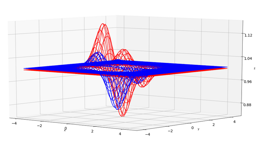
The next graph shows the sum, i.e. the full “cost function”, in green in comparison to the (vertically shifted and scaled) original functions.

Also here you clearly see the differences in the minimas’ positions. What does this mean for gradient descent?

Firstly, the contour lines on the total cost function would deviate from the ones on the cost function hyperplanes of our 2 batches. So would the directions of the different gradients at the point presently reached in the parameter space during optimization! Working with batches therefore means jumping around on the surface of the total cost function a bit erratically and not precisely along the direction of steepest descent there. By the way: This behavior can be quite helpful to overcome local minima.

Secondly, in our simplified example we would in the end not converge completely, but jump or circle around the minimum of the total cost function. Reason: Each batch forces the weight corrections for x,y into different directions namely those of
its own minimum. So, a weight correction induced by one bath would be countered by corrections imposed by the optimization for the other batch. (Regarding MNIST it would e.g. be interesting to run a batch with handwritten digits of Europeans against a batch with digits written by Americans and see how the weights differ after gradient descent has converged for each batch.)

This makes us understand multiple things:

  • Mini-batches should be built with a statistical distribution of records and their composition should be changed statistically from epoch to epoch.
  • We need a criterion to stop iterating over too many epochs senselessly.
  • We should investigate whether the number and thus the size of mini-batches influences the results of EBP.
  • At the end of an optimization run we could invest in some more iterations not for the batches, but for the full cost function of all training records and see if we can get a little deeper into the minimum of this total cost function.
  • We should analyze our batches – if we keep them up and do not create them statistically anew at the beginning of each epoch – for special data records whose properties are off of the normal – and maybe eliminate those data records.

Repetition: Why Back-propagation of 2 dimensional matrices and not vectors?

The step wise matrix operations of EBP are to be performed according to a scheme with the following structure:

  • On a given layer N apply a layer specific matrix “NW.T” (depending on the weights there) by some operational rule on some matrix “(N+1)δS“, which contains some data already calculated for layer (N+1).
  • Take the results and modify it properly by multiplying it element-wise with some other matrix ND (containing derivative expressions for the activation function) until you get a new NδS.
  • Get partial derivatives of the cost function with respect to the weights on layer (N-1) by a further matrix operation of NδS on a matrix with output values (N-1)A.TS on layer (N-1).
  • Proceed to the next layer in backward direction.

The input into this process is a matrix of error-dependent quantities, which are defined at the output layer. These values are then back-propagated in parallel to the inner layers of our MLP.

Now, why do we propagate data matrices and not just data vectors? Why are we allowed to combine so many different multiplications and summations described in the last article when we deal with partial derivatives with respect to variables deep inside the network?

The answer to the first question is numerical efficiency. We operate on all data records of a mini-batch in parallel; see the PDF. The answer to the second question is 2-fold:

  • We are allowed to perform so many independent operations because of the linear structure of our cost-functions with respect to contributions coming from the records of a mini-batch and the fact that we just apply linear operations between layers during forward propagation. All contributions – however non-linear each may be in itself – are just summed up. And propagation itself between layers is defined to be linear.
  • The only non-linearity occurring – namely in the form of non-linear activation functions – is to be applied just on layers. And there it works only node-wise! We do not
    couple values for nodes on one and the same layer.

In this sense MLPs are very simple by definition – although they may look complex! (By the way and if you wonder why MLPs are nevertheless so powerful: One reason has to do with the “Universal Approximation Theorem”; see the literature hint at the end.)

Consequence of the simplicity: We can deal with δ-values (see the PDF) for both all nodes of a layer and all records of a mini-batch in parallel.

Results derived in the last article would change dramatically if we had rules that coupled the Z- or A-values of different nodes! E.g. if the squared value at node 7 in layer X must always be the sum of squared values at nodes 5 an 6. Believe me: There are real networks in this world where such a type of node coupling occurs – not only in physics.

Note: As we have explained in the PDF, the nodes of a layer define one dimension of the NδS“-matrices,
the number of mini-batch records the other. The latter remains constant. So, during the process the δ-matrices change only one of their 2 dimensions.

Some possible pitfalls to tackle before EBP-coding

Now, my friends, we can happily start coding … Nope, there are actually some minor pitfalls, which we have to explain first.

Special cost-, activation- and output-functions

I refer to the PDF mentioned above and its formulas. The example explained there referred to the “Log Loss” function, which we took as an example cost function. In this case the outδS and the 3δS-terms at the nodes of the outermost layer turned out to be quite simple. See formula (21), (22), (26) and (27) in the PDF.

However, there may be other cost functions for which the derivative with respect to the output vector “a” at the outermost nodes is more complicated.

In addition we may have other output or activation functions than the sigmoid function discussed in the PDF’s example. Further, the output function may differ from the activation function at inner layers. Thus, we find that the partial derivatives of these functions with respect to their variables “z” must be calculated explicitly and as needed for each layer during back propagation; i.e., we have to provide separate and specific functions for the provision of the required derivatives.

At the outermost layer we apply the general formulas (84) to (88) with matrix ED containing derivatives of the output-function Eφ(z) with respect to the input z to find EδS with E marking the outermost layer. Afterwards, however, we apply formula (92) – but this time with D-elements referring to derivatives of the standard activation-function φ used at nodes of inner layers.

The special case of the Log Loss function and other loss functions with critical denominators in their derivative

Formula (21) shows something interesting for the quantity outδS, which is a starting point for backward propagation: a denominator depending on critical factors, which directly involve output “a” at the outer nodes or “a” in a difference term. But in our one-hot-approach “a” may become zero or come close to it – during training by accident or by convergence! This is a dangerous thing; numerically we absolutely want to avoid any division by zero or by small numbers close to the numerical accuracy of a programming language.

What mathematically saves us in the special case of Log Loss are formulas (26) and (27), where due to some “magic” the dangerous denominator is cancelled by a corresponding factor in the numerator when we evaluate EδS.

In the general case, however,
we must investigate what numerical dangers the functional form of the derivative of the loss function may bring with it. In the end there are two things we should do:

  • Build a function to directly calculate EδS and put as much mathematical knowledge about the involved functions and operations into it as possible, before employing an explicit calculation of values of the cost function’s derivative.
  • Check the involved matrices, whose elements may appear in denominators, for elements which are either zero or close to it in the sense of the achievable accuracy.

For our program this means: Whether we calculate the derivative of a cost function to get values for “outδS” will depend on the mathematical nature of the cost function. In case of Log Loss we shall avoid it. In case of MSE we shall perform the numerical operation.

Handling of bias nodes

A further complication of our aspired coding has its origin in the existence of bias nodes on every inner layer of the MLP. A bias node of a layer adds an additional degree of freedom whilst adjusting the layer’s weights; a bias node has no input, it produces only a constant output – but is connected with weights to all normal nodes of the next layer.

Some readers who are not so familiar with “artificial neural networks” may ask: Why do we need bias nodes at all?

Well, think about a simple matrix operation on a 2 dim-vector; it changes its direction and length. But if we want to approximate a function for regression or a separation hyperplanes for classification by a linear operation then we need another element which corresponds to a constant translation part in a linear transformation: z = w1*x1 + w2*x2 + const.. Take a simple function y=w*x + c. The “c” controls where the line crosses the y axis. We need such a parameter if our line should separate clusters of points separably distributed somewhere in the (x,y)-plane; the w is not sufficient to orientate and position the hyperplane in the (x,y)-plane.

This very basically what bias neurons are good for regarding the basically linear operation between two MLP-layers. They add a constant to an otherwise linear transformation.

Do we need a bias node on all layers? Definitely on the input layer. However, on the hidden layers a trained network could by learning evolve weights in such a way that a bias neuron comes about – with almost zero weights on one side. At least in principle; however, we make it easier for the MLP to converge by providing explicit “bias” neurons.

What did we do to account for bias nodes in our Python code so far? We extended the matrices describing the output arrays ay_A_out of the activation function (for input ay_Z_in) on the input and all hidden layers by elements of an additional row. This was done by the method “add_bias_neuron_to_layer()” – see the codes given in article III.

The important point is that our weight matrices already got a corresponding dimension when we built them; i.e. we defined weights for the bias nodes, too. Of course, during optimization we must calculate partial derivatives of the cost function with respect to these weights.

The problem is:

We need to back propagate a delta-matrix Nδ for layer N via
( (NW.T).dot(Nδ) ). But then we can not apply a simple element-wise matrix multiplication with the (N-1)D(z)-matrix at layer N-1. Reason: The dimensions do not fit, if we calculate the elements of D only for the existing Z-Values at layer N-1.

There are two solutions for coding:

  • We can add a row artificially and intermediately to the Z-matrix to calculate the D-matrix, then calculate NδS as
    ( (NW.T).dot(Nδ) ) * (N_1)D
    and eliminate the first artificial row appearing in NδS afterwards.
  • The other option is to reduce the weight-matrix (NW) by a row intermediately and restore it again afterwards.

What we do is a matter of efficiency; in our coding we shall follow the first way and test the difference to the second way afterwards.

Check the matrix dimensions

As all steps to back-propagate and to circumvent the pitfalls require a bit of matrix wizardry we should at least check at every step during EBP backward-propagation that the dimensions of the involved matrices fit each other.

Outlook

Guys, after having explained some of the matrix math in the previous article of this series and the problems we have to tackle whilst programming the EBP-algorithm we are eventually well prepared to add EBP-methods to our Python class for MLP simulation. We are going to to this in the next article:
A simple program for an ANN to cover the Mnist dataset – VIII – coding Error Backward Propagation

Literature

“Machine Learning – An Applied Mathematics Introduction”, Paul Wilmott, 2019, Panda Ohana Publishing

A simple Python program for an ANN to cover the MNIST dataset – II – initial random weight values

In this article series we are going to build a relatively simple Python class for the simulation of a “Multilayer Perceptron” [MLP]. A MLP is a simple form of an “artificial neural network” [ANN] with multiple layers of neurons. It has three characteristic properties: (1) Only connections between nodes of neighboring layers are allowed. (2) Information transport occurs in one forward direction. We speak of a “forward propagation of input information” through the ANN. (3) Neighboring layers are densely connected; a node of layer L_n is connected to all nodes of layer L_(n+1).

The firsts two points mean simplifications: According to (1) we do not consider so called cascaded networks. According to (2) no loops occur in the information transport. The third point, however, implies a lot of mathematical operations – not only during forward propagation of information through the ANN, but also – as we shall see – during the training and optimization of the network where we will back propagate “errors” from the output to the input layers. But for the next articles we need to care about simpler things first.

We shall use our MLP for classification tasks. Our first objective is to apply it to the MNIST dataset. In my last article

A simple program for an ANN to cover the Mnist dataset – I – a starting point

I presented already some code for the “__init__”-function on some other methods of our Python class. It enabled us to import MNIST data and split them in to a set of training and a set of test samples. Note that this is a standard approach in Machine Learning: You train on one set of data samples, but you test the classification or regression abilities of your ANN on a separate disjunctive data set.

In the present article we shall extend the functionality of our class: First we shall equip our network layers with a defined number of nodes. Then we shall provide statistical initial values for the “weights” describing the forward transport of information along the connections between the layers of our network.

Present status of our function “__init__”

The present status of our __init__function is:

    def __init__(self, 
                 my_data_set = "mnist", 
                 n_hidden_layers = 1, 
                 ay_nodes_layers = [0, 100, 0], # array which should have as much elements as n_hidden + 2
                 n_nodes_layer_out = 10,  # expected number of nodes in output layer 
                                                  
                 my_activation_function = "sigmoid", 
                 my_out_function        = "sigmoid",   
                 
                 n_mini_batch = 1000,  # number of data elements in a mini-batch 
                 
                 vect_mode = 'cols', 
                 
                 figs_x1=12.0, figs_x2=8.0, 
                 legend_loc='upper right',
                 
                 b_print_test_data = True
                 
                 ):
        '''
        Initialization of MyANN
        Input: 
            data_set: type of dataset; so far only the "mnist", "mnist_784" datsets are known 
                      We use this information to prepare the input data and learn about the feature dimension. 
                      This info is used in preparing the size of the input layer.     
            n_hidden_layers = number of hidden layers => between input layer 0 and output layer n 

            ay_nodes_layers = [0, 100, 0 ] : We set the number of nodes in input layer_0 and the output_layer to zero 
                              Will be set to real number afterwards by infos from the input dataset. 
       
                       All other numbers are used for the node numbers of the hidden layers.
            n_nodes_out_layer = expected number of nodes in the output layer (is checked); 
                                this number corresponds to the number of categories NC = number of labels to be distinguished
            
            my_activation_function : name of the activation function to use 
            my_out_function : name of the "activation" function of the last layer which produces the output values 
            
            n_mini_batch : Number of elements/samples in a mini-batch of training dtaa 
            
            vect_mode: Are 1-dim data arrays (vctors) ordered by columns or rows ?

            figs_x1=12.0, figs_x2=8.0 : Standard sizing of plots , 
            legend_loc='upper right': Position of legends in the plots
            
            b_print_test_data: Boolean variable to control the print out of some tests data 
             
         '''
        
        # Array (Python list) of known input data sets 
        self._input_data_sets = ["mnist", "mnist_784", "mnist_keras"]  
        self._my_data_set = my_data_set
        
        # X, y, X_train, y_train, X_test, y_test  
            # will be set by analyze_input_data 
            # X: Input array (2D) - at present status of MNIST image data, only.    
            # y: result (=classification data) [digits represent categories in the case of Mnist]
        self._X       = None 
        self._X_train = None 
        self._X_test  = None   
        self._y       = None 
        self._y_train = None 
        self._y_test  = None
        
        # relevant dimensions 
        # from input data information;  will be set in handle_input_data()
        self._dim_sets     = 0  
        self._dim_features = 0  
        self._n_labels     = 0   # number of unique labels - will be extracted from y-data 
        
        # Img sizes 
        self._dim_img      = 0 # should be sqrt(dim_features) - we assume square like images  
        self._img_h        = 0 
        self._img_w        = 0 
        
        # Layers
        # ------
        # number of hidden layers 
        self._n_hidden_layers = n_hidden_layers
        # Number of total layers 
        self._n_total_layers = 2 + self._n_hidden_layers  
        # Nodes for hidden layers 
        self._ay_nodes_layers = np.array(ay_nodes_layers)
        # Number of nodes in output layer - will be checked against information from target arrays
        self._n_nodes_layer_out = n_nodes_layer_out
        
        
        # Weights 
        # --------
        # empty List for all weight-matrices for all layer-connections
        # Numbering : 
        # w[0] contains the weight matrix which connects layer 0 (input layer ) to hidden layer 1 
        # w[1] contains the weight matrix which connects layer 1 (input layer ) to (hidden?) layer 2 
        self._ay_w = []  
        
        # Known Randomizer methods ( 0: np.random.randint, 1: np.random.uniform )  
        # ------------------
        self.__ay_known_randomizers = [0, 1]

        # Types of activation functions and output functions 
        # ------------------
        self.__ay_activation_functions = ["sigmoid"] # later also relu 
        self.__ay_output_functions     = ["sigmoid"] # later also softmax 
        
        # the following dictionaries will be used for indirect function calls 
        self.__d_activation_funcs = {
            'sigmoid': self._sigmoid, 
            'relu':    self._relu
            }
        self.__d_output_funcs = { 
            'sigmoid': self._sigmoid, 
            'softmax': self._softmax
            }  
          
        # The following variables will later be set by _check_and set_activation_and_out_functions()            
        
self._my_act_func = my_activation_function
        self._my_out_func = my_out_function
        self._act_func = None    
        self._out_func = None    

        # number of data samples in a mini-batch 
        self._n_mini_batch = n_mini_batch


        # print some test data 
        self._b_print_test_data = b_print_test_data

        # Plot handling 
        # --------------
        # Alternatives to resize plots 
        # 1: just resize figure  2: resize plus create subplots() [figure + axes] 
        self._plot_resize_alternative = 1 
        # Plot-sizing
        self._figs_x1 = figs_x1
        self._figs_x2 = figs_x2
        self._fig = None
        self._ax  = None 
        # alternative 2 does resizing and (!) subplots() 
        self.initiate_and_resize_plot(self._plot_resize_alternative)        
        
        
        # ***********
        # operations 
        # ***********
        # check and handle input data 
        self._handle_input_data()
        
        print("\nStopping program regularily")
        sys.exit()

 
The kind reader may have noticed that this is not exactly what was presented in the last article. I have introduced two additional parameters and corresponding class attributes:
“b_print_test_data” and “n_mini_batch”.

The first of these parameters controls whether we print out some test data or not. The second parameter controls the number of test samples dealt with in parallel during propagation and optimization via the so called “mini-batch-approach” mentioned in the last article.

Setting node numbers of the layers

We said in the last article that we would provide the numbers of nodes of the ANN layers via a parameter list “ay_nodes_layers”. We set the number of nodes for the input and the output layer, i.e. the first number and the last number in the list, to “0” in this array because these numbers are determined by properties of the input data set – here the MNIST dataset.

All other numbers in the array determine the amount of nodes of the hidden layers in consecutive order between the input and the output layer. So, the number at ay_nodes_layers[1] is the number of nodes in the first hidden layer, i.e. the layer which follows after the input layer.

In the last article we have understood already that the number of nodes in the input layer should be equal to the full number of “features” of our input data set – 784 in our case. The number of nodes of the output layer must instead be determined from the number of categories in our data set. This is equivalent to the number of distinct labels in the set of training data represented by an array “_y_train” (in case of MNIST: 10).

We provide three methods to check the node numbers defined by the user, set the node numbers for the input and output layers and print the numbers.

    # Method which checks the number of nodes given for hidden layers 
    def _check_layer_and_node_numbers(self): 
        try: 
            if (self._n_total_layers != (self._n_hidden_layers + 2)): 
                raise ValueError
        except ValueError:
            print("The assumed total number of layers does not fit the number of hidden layers + 2") 
            sys.exit()   
        try: 
            if (len(self._ay_nodes_layers) != (self._n_hidden_layers + 2)): 
                raise ValueError
        except ValueError:
            print("The number of elements in the array for layer-nodes does not fit the number of hidden layers + 2") 
            sys.exit(1)   
    
    # Method which sets the number of nodes of the input and the layer 
    def _set_nodes_for_input_output_layers(self): 
        
        # Input layer: for the input layer we do 
NOT take into account a bias node 
        self._ay_nodes_layers[0] = self._dim_features 
                
        # Output layer: for the output layer we check the number of unique values in y_train
        try: 
            if ( self._n_labels != (self._n_nodes_layer_out) ): 
                raise ValueError
        except ValueError:
            print("The unique elements in target-array do not fit number of nodes in the output layer") 
            sys.exit(1)   
        self._ay_nodes_layers[self._n_total_layers - 1] = self._n_labels     


    # Method which prints the number of nodes of all layers 
    def _show_node_numbers(self): 
        print("\nThe node numbers for the " + str(self._n_total_layers) + " layers are : ")
        print(self._ay_nodes_layers)

 
The code should be easy to understand. self._dim_features was set in the method “_common_handling_of mnist()” discussed in the last article. It was derived from the shape of the input data array _X_train. The number of unique labels was evaluated by the method “_get_num_labels()” – also discussed in the last article.

Note: The initial node numbers DO NOT include a bias node, yet.

If we extend the final commands in the “__init__”-function by :

        # ***********
        # operations 
        # ***********
        # check and handle input data 
        self._handle_input_data()

        # check consistency of the node-number list with the number of hidden layers (n_hidden)
        self._check_layer_and_node_numbers()
        # set node numbers for the input layer and the output layer
        self._set_nodes_for_input_output_layers() 
        self._show_node_numbers() 
        
        print("\nStopping program regularily")
        sys.exit()


By testing our additional code in a Jupyter notebook we get a corresponding output for

ANN = myann.MyANN(my_data_set="mnist_keras", n_hidden_layers = 2, 
                     ay_nodes_layers = [0, 100, 50, 0], 
                     n_nodes_layer_out = 10,  
                     vect_mode = 'cols', 
                     figs_x1=12.0, figs_x2=8.0, 
                     legend_loc='upper right',
                     b_print_test_data = False
                     )

of:

The node numbers for the 4 defined layers are: 
[784 100  50  10]

Good!

Setting initial random numbers for the weights

Initial values for the ANN weights have to be given as matrices, i.e. 2-dim arrays. However, the randomizer functions provided by Numpy give you vectors as output. So, we need to reshape such vectors into the required form.

First we define a method to provide random floating point and integer numbers:

 
    # ---
    # method to create an array of randomized values
    def _create_vector_with_random_values(self, r_low=None, r_high=None, r_size=None, randomizer=0 ):   
        '''
        Method to create a vector of length "r_size" with "random values" in [r_low, r_high] 
        generated by method "randomizer" 
        Input: 
        ramdonizer : integer which sets randomizer method; presently only 
            0: np.random.uniform 
            1: np.randint     
        [r_low, r_high]: range of the random numbers to be created
        r_size: Size of output array 
        Output: A 1-dim numpy array of length rand-size - produced as a class member 
        '''
        # check parameters
        try: 
            if (r_low==None or r_high == None or r_size == None ): 
                raise ValueError
        except ValueError:
            print("One of 
the required parameters r_low, r_high, r_size has not been set") 
            sys.exit(1)   
        
        rmizer = int(randomizer)
        try: 
            if (rmizer not in self.__ay_known_randomizers): 
                raise ValueError
        except ValueError:
            print("randomizer not known") 
            sys.exit(1)   
        
        # 2 randomizers (so far)
        if (rmizer == 0): 
            ay_r_out = np.random.randint(int(r_low), int(r_high), int(r_size))
        if (rmizer == 1):
            ay_r_out = np.random.uniform(r_low, r_high, size=int(r_size))
            
        return ay_r_out     

 
Presently, we can only use two randomizer functions to be used – numpy.random.randint and numpy.random.uniform. The first one provides random integer values, the other one floating point values – both within a defined interval. The parameter “r_size” defines how many random numbers shall be created and put into an array. The code requires no further explanation.

Now, we define two methods to create the weight matrices for the connections

  • between the input layer L0 to the first hidden layer,
  • between further hidden layers and eventually between the last hidden layer and the output layer

As we allow for all possible connections between nodes the dimensions of the matrices are determined by the numbers of nodes in the connected neighboring layers. Each node of a layer L_n cam be connected to each node of layer L_(n+1). Our methods are:

 
    # Method to create the weight matrix between L0/L1
    # ------
    def _create_WM_Input(self):
        '''
        Method to create the input layer 
        The dimension will be taken from the structure of the input data 
        We need to fill self._w[0] with a matrix for conections of all nodes in L0 with all nodes in L1
        We fill the matrix with random numbers between [-1, 1] 
        '''
        # the num_nodes of layer 0 should already include the bias node 
        num_nodes_layer_0 = self._ay_nodes_layers[0]
        num_nodes_with_bias_layer_0 = num_nodes_layer_0 + 1 
        num_nodes_layer_1 = self._ay_nodes_layers[1] 
        
        # fill the matrix with random values 
        rand_low  = -1.0
        rand_high = 1.0
        rand_size = num_nodes_layer_1 * (num_nodes_with_bias_layer_0) 
        
        randomizer = 1 # method np.random.uniform   
        
        w0 = self._create_vector_with_random_values(rand_low, rand_high, rand_size, randomizer)
        w0 = w0.reshape(num_nodes_layer_1, num_nodes_with_bias_layer_0)
        
        # put the weight matrix into array of matrices 
        self._ay_w.append(w0.copy())
        print("\nShape of weight matrix between layers 0 and 1 " + str(self._ay_w[0].shape))


    # Method to create the weight-matrices for hidden layers 
    def _create_WM_Hidden(self):
        '''
        Method to create the weights of the hidden layers, i.e. between [L1, L2] and so on ... [L_n, L_out] 
        We fill the matrix with random numbers between [-1, 1] 
        '''
        
        # The "+1" is required due to range properties ! 
        rg_hidden_layers = range(1, self._n_hidden_layers + 1, 1)

        # for random operation 
        rand_low  = -1.0
        rand_high = 1.0
        
        for i in rg_hidden_layers: 
            print ("Creating weight matrix for layer " + str(i) + " to layer " + str(i+1) )
            
            num_nodes_layer = self._ay_nodes_layers[i] 
            num_nodes_with_bias_layer = num_nodes_layer + 1 
            
            # the number of the next layer is taken without the bias node!
            num_nodes_layer_
next = self._ay_nodes_layers[i+1]
            
            # assign random values  
            rand_size = num_nodes_layer_next * num_nodes_with_bias_layer   
            
            randomizer = 1 # np.random.uniform
            
            w_i_next = self._create_vector_with_random_values(rand_low, rand_high, rand_size, randomizer)   
            w_i_next = w_i_next.reshape(num_nodes_layer_next, num_nodes_with_bias_layer)
            
            # put the weight matrix into our array of matrices 
            self._ay_w.append(w_i_next.copy())
            print("Shape of weight matrix between layers " + str(i) + " and " + str(i+1) + " = " + str(self._ay_w[i].shape))

 
Three things may need explanation:

  • The first thing is the inclusion of a bias-node in all layers. A bias node only provides input to the next layer but does not receive input from a preceding layer. It gives an additional bias to the input a layer provides to a neighbor layer. (Actually, it provides an additional degree of freedom for the optimization process.) So, we include connections from a bias-node of a layer L_n to all nodes (without the bias-node) in layer L_(n+1).
  • The second thing is the reshaping of the vector of random numbers into a matrix. Of course, the dimension of the vector of random numbers must fit the product of the 2 matrix dimensions. Note that the first dimension always corresponds to number of nodes in layer L_(n+1) and the second dimension to the number of nodes in layer L_n (including the bias-node)!
    We need this special form to support the vectorized propagation properly later on.
  • The third thing is that we save our (Numpy) weight matrices as elements of a Python list.

In my opinion this makes the access to these matrices flexible and easy in the case of multiple hidden layers.

Setting the activation and output functions

We must set the activation and the output function. This is handled by a method “_check_and_set_activation_and_out_functions()”.

 
    def _check_and_set_activation_and_out_functions(self):
        # check for known activation function 
        try: 
            if (self._my_act_func not in self.__d_activation_funcs ): 
                raise ValueError
        except ValueError:
            print("The requested activation function " + self._my_act_func + " is not known!" )
            sys.exit()   
        # check for known output function 
        try: 
            if (self._my_out_func not in self.__d_output_funcs ): 
                raise ValueError
        except ValueError:
            print("The requested output function " + self._my_out_func + " is not known!" )
            sys.exit()   
             
        # set the function to variables for indirect addressing 
        self._act_func = self.__d_activation_funcs[self._my_act_func]
        self._out_func = self.__d_output_funcs[self._my_out_func]
        
        if self._b_print_test_data:
            z = 7.0
            print("\nThe activation function of the standard neurons was defined as \""  + self._my_act_func + '"') 
            print("The activation function gives for z=7.0:  " + str(self._act_func(z))) 
            print("\nThe output function of the neurons in the output layer was defined as \"" + self._my_out_func + "\"") 
            print("The output function gives for z=7.0:  " + str(self._out_func(z))) 


It requires not much of an explanation. For the time being we just rely on the given definition of the “__init__”-interface, which sets both to “sigmoid()”. The internal dictionaries __d_activation_funcs[] and __d_output_funcs[] provide the functions to
internal variables (indirect addressing).

Some test output

A test output for the enhanced code

 
        # ***********
        # operations 
        # ***********
        # check and handle input data 
        self._handle_input_data()

        # check consistency of the node-number list with the number of hidden layers (n_hidden)
        self._check_layer_and_node_numbers()
        # set node numbers for the input layer and the output layer
        self._set_nodes_for_input_output_layers() 
        self._show_node_numbers() 

        # create the weight matrix between input and first hidden layer 
        self._create_WM_Input() 
        # create weight matrices between the hidden layers and between tha last hidden and the output layer 
        self._create_WM_Hidden() 

        # check and set activation functions 
        self._check_and_set_activation_and_out_functions()

        print("\nStopping program regularily")
        sys.exit()


and a Jupyter cell

gives :

The shapes of the weight matrices correspond correctly to the numbers of nodes in the 4 layers defined. (Do not forget about the bias-nodes!).

Conclusion

We have reached a status where our ANN class can read in the MNIST dataset and set initial random values for the weights. This means that we can start to do some more interesting things. In the next article

A simple program for an ANN to cover the Mnist dataset – III – forward propagation

we shall program the “forward propagation”. We shall perform the propagation for a mini-batch of many data samples in one step. We shall see that this is a very simple task, which only requires a few lines of code.