
I sit in front of my old laptop and want to pre-process data of a pool of scanned texts for an analysis with ML and conventional algorithms. One of the tasks will be to correct at least some wrongly scanned words by “brute force” methods. A straight forward approach is to compare “3-character-gram” segments of the texts’ distinguished words (around 1.9 million) with the 3-char-gram patterns of the words of a reference vocabulary. The vocabulary I use contains around 2.7 million German words.
I started today with a 3-char-gram segmentation of the vocabulary – just to learn that tackling this problem with Pandas and Python pretty soon leads to a significant amount of RAM consumption. RAM is limited on my laptop (16 GB), so I have to keep memory requirements low. In this post I discuss some elementary Pandas tricks which helped me reduce memory consumption.
The task
I load my vocabulary from a CSV file into a Pandas dataframe named “dfw_uml“. The structure of the data is as follows:
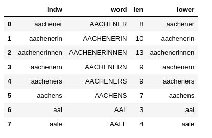
The “indw”-column is identical to the “lower”-column. “indw” allows me to quickly use the “lower” version of the words as an (unique) index instead of an integer index. (This is a very useful option regarding some analysis. Note: As long as the string-based index is unique a hash function is used to make operations using a string-based index very fast.)
For all the words in the vocabulary I want to get all their individual 3-char-gram segments. “All” needs to be qualified: When you split a word in 3-char-grams you can do this with an overlap of the segments or without. Similar to filter kernels of CNNs I call the character-shift of consecutive 3-char-grams against each other “stride“.
Let us look at a short word like “angular” (with a length “len” = 7 characters). How many 3-char-grams do we get with a stride of 1? This depends on a padding around the word’s edges with special characters. Let us say we allow for a left-padding of 2 characters “%” on the left side of the word and 2 characters “#” on the right side. (Assuming that these characters are no parts of the words themselves. Then, with a stride of “1”, the 3-char-grams are :
‘%%a’, ‘%an’, ‘ang’, ‘ngu’, ‘gul’, ‘ula’, ‘lar’, ‘ar#’, ‘r##’
I.e., we get len+2 (=9) different 3-char-grams.
However, with a stride of 3 and a left-padding of 0 we get :
‘ang’, ‘ula’, ‘r##’
I.e., len/3 + 1 (=3) different 3-char-grams. (Whether we need an additional 3-char-ram depends on the division rest len%3). On the right-hand side of the word we have to allow for filling the rightmost 3-char-gram with our extra character “#”.
The difference in the total number of 3-char-grams is substantial. And it becomes linearly bigger with the word-length.
In a German vocabulary many quite long words (composita) may appear. In my vocabulary the longest word has 58 characters:
“telekommunikationsnetzgeschaeftsfuehrungsgesellschaft”
(with umlauts ä and ü written as ‘ae’ and ‘ue’, respectively). So, we talk about 60 or 20 additional columns required for “all” 3-char-grams.
So, choosing a suitable stride is an important factor to control memory consumption. But for some kind of analysis you may just want to limit the number (num_gram) of 3-char-grams for your analysis. E.g. you may set num_grams = 20.
When working with a Pandas table-like data structure it seems logical to arrange all of the 3-char-grams in form of different columns. Let us take a number of 20 columns
for different 3-char-grams as an objective for this article. We can create such 3-char-grams for all vocabulary words either with a “stride=3” or “stride = 1” and “num_grams = 20”. I pick the latter option.
Which padding and stride values are reasonable?
Padding on the right side of a word is in my opinion always reasonable when creating the 3-char-grams. You will see from the code in the next section how one creates the right-most 3-char-grams of the vocabulary words efficiently. On the left side of a word padding may depend on what you want to analyze. The following stride and left-padding combinations seem reasonable to me for 3-char-grams:
- stride = 3, left-padding = 0
- stride = 2, left-padding = 0
- stride = 2, left-padding = 2
- stride = 1, left-padding = 2
- stride = 1, left-padding = 1
- stride = 1, left-padding = 0
Code to create 3-char-grams
The following function builds the 3-char-grams for the different combinations.
def create_3grams_of_voc(dfw_words, num_grams=20,
                         padding=2, stride=1,
                         char_start='%', char_end='#', b_cpu_time=True):

    cpu_time = 0.0
    if b_cpu_time:
        v_start_time = time.perf_counter()

    # Some checks
    if stride > 3:
        print('stride > 3 cannot be handled of this function for 3-char-grams')
        return dfw_words, cpu_time
    if stride == 3 and padding > 0:
        print('stride == 3 should be used with padding=0 ')
        return dfw_words, cpu_time
    if stride == 2 and padding == 1:
        print('stride == 2 should be used with padding=0, 2 - only')
        return dfw_words, cpu_time

    st1 = char_start
    st2 = 2*char_start

    # begin: starting index for loop below
    begin = 0
    if stride == 3:
        begin = 0
    if stride == 2 and padding == 2:
        dfw_words['gram_0'] = st2 + dfw_words['lower'].str.slice(start=0, stop=1)
        begin = 1
    if stride == 2 and padding == 0:
        begin = 0
    if stride == 1 and padding == 2:
        dfw_words['gram_0'] = st2 + dfw_words['lower'].str.slice(start=0, stop=1)
        dfw_words['gram_1'] = st1 + dfw_words['lower'].str.slice(start=0, stop=2)
        begin = 2
    if stride == 1 and padding == 1:
        dfw_words['gram_0'] = st1 + dfw_words['lower'].str.slice(start=0, stop=2)
        begin = 1
    if stride == 1 and padding == 0:
        begin = 0

    # for num_grams == 20 we have to create elements up to and including gram_21 (range -> 22)

    # Note that the operations in the loop occur column-wise, i.e vectorized
    # => You cannot make them row dependend
    # We are lucky that slice returns ''
    for i in range(begin, num_grams+2):
        col_name = 'gram_' + str(i)

        sl_start = i*stride - padding
        sl_stop  = sl_start + 3

        dfw_words[col_name] = dfw_words['lower'].str.slice(start=sl_start, stop=sl_stop)
        dfw_words[col_name] = dfw_words[col_name].str.ljust(3, '#')

    # We are lucky that nothing happens if not required to fill up
    #for i in range(begin, num_grams+2):
    #    col_name = 'gram_' + str(i)
    #    dfw_words[col_name] = dfw_words[col_name].str.ljust(3, '#')

    if b_cpu_time:
        v_end_time = time.perf_counter()
        cpu_time   = v_end_time - v_start_time

    return dfw_words, cpu_time
The only noticeable thing about this code is the vectorized handling of the columns. (The whole setup of the 3-char-gram columns still requires around 51 secs on my laptop).
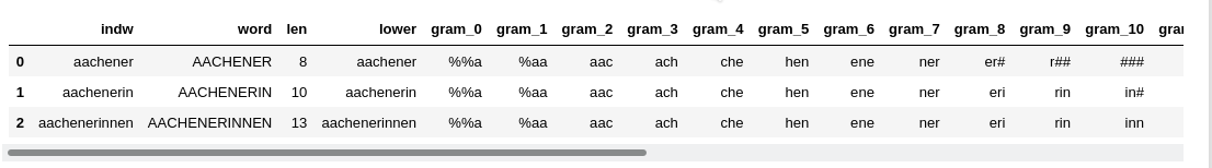
We call the function above for stride=1, padding=2, num_grams=20 by the following code in a
Jupyter cell:
num_grams = 20; stride = 2; padding = 2
dfw_uml, cpu_time = create_3grams_of_voc(dfw_uml, num_grams=num_grams, padding=padding, stride=stride)
print("cpu_time = ", cpu_time)
print()
dfw_uml.head(3)
RAM consumption
Let us see how the memory consumption looks like. After having loaded all required libraries and some functions my Jupyter plugin “jupyter-resource-usage” for memory consumption shows: “Memory: 208.3 MB“.
When I fill the Pandas dataframe “dfw_uml” with the vocabulary data this number changes to: “Memory: 915 MB“.
Then I create the 3-char-gram-columns for “num_grams = 20; stride = 1; padding = 2” and get:
The memory jumped to “Memory: 4.5 GB“. The OS wth some started servers on the laptop takes around 2.6 GB. So, we have already consumed around 45% of the available RAM.
Looking at details by
dfw_uml.info(memory_usage='deep')
shows
<class 'pandas.core.frame.DataFrame'>
RangeIndex: 2700936 entries, 0 to 2700935
Data columns (total 26 columns):
 #   Column   Dtype
---  ------   -----
 0   indw     object
 1   word     object
 2   len      int64
 3   lower    object
 4   gram_0   object
 5   gram_1   object
 6   gram_2   object
 7   gram_3   object
 8   gram_4   object
 9   gram_5   object
 10  gram_6   object
 11  gram_7   object
 12  gram_8   object
 13  gram_9   object
 14  gram_10  object
 15  gram_11  object
 16  gram_12  object
 17  gram_13  object
 18  gram_14  object
 19  gram_15  object
 20  gram_16  object
 21  gram_17  object
 22  gram_18  object
 23  gram_19  object
 24  gram_20  object
 25  gram_21  object
dtypes: int64(1), object(25)
memory usage: 4.0 GB
The memory consumption due to our expanded dataframe is huge. No wonder with around 59.4 million string like entries in the dataframe! With Pandas we have no direct option of telling the columns to use specific 3 character columns. For strings Pandas instead uses a flexible datatype “object“.
Reducing memory consumption by using datatype “category”
Looking at the data we get the impression that one should be able to reduce the amount of required memory because the entries in all of the 3-char-gram-columns are non-unique. Actually, the 3-char-grams mark major groups of words (probably in a typical way for a given western language).
We can get the number of unique 3-char-grams in a column with the following code snippet:
li_unique = []
for i in range(2,22):
    col_name     = 'gram_' + str(i)
    count_unique = dfw_uml[col_name].nunique()
    li_unique.append(count_unique)
print(li_unique)
Giving for our 21 columns:
[3068, 4797, 8076, 8687, 8743, 8839, 8732, 8625, 8544, 8249, 7829, 7465, 7047, 6700, 6292, 5821, 5413, 4944, 4452, 3989]
Compared to 2.7 million rows these numbers are relatively small. This is where the datatype (dtype) “category” comes handy. We can transform the dtype of the dataframe columns by
for i in range(0,22):
    col_name     = 'gram_' + str(i)
    dfw_uml[col_name] = dfw_uml[col_name].astype('category')
“dfw_uml.info(memory_usage=’deep’)” afterwards gives us:
<class 'pandas.core.frame.DataFrame'>
RangeIndex: 2700936 entries, 0 to 2700935
Data columns (total 26 columns):
 #   Column   Dtype
---  ------   -----
 0   indw     object
 1   word     object
 2   len
int64
 3   lower    object
 4   gram_0   category
 5   gram_1   category
 6   gram_2   category
 7   gram_3   category
 8   gram_4   category
 9   gram_5   category
 10  gram_6   category
 11  gram_7   category
 12  gram_8   category
 13  gram_9   category
 14  gram_10  category
 15  gram_11  category
 16  gram_12  category
 17  gram_13  category
 18  gram_14  category
 19  gram_15  category
 20  gram_16  category
 21  gram_17  category
 22  gram_18  category
 23  gram_19  category
 24  gram_20  category
 25  gram_21  category
dtypes: category(22), int64(1), object(3)
memory usage: 739.9 MB
Just 740 MB!
Hey, we have reduced the required memory for the dataframe by more than a factor of 4!/
Read in data from CSV with already reduced memory
We can now save the result of our efforts in a CSV-file by
# the following statement just helps to avoid an unnamed column during export
dfw_uml = dfw_uml.set_index('indw')
# export to csv-file
export_path_voc_grams = '/YOUR_PATH/voc_uml_grams.csv'
dfw_uml.to_csv(export_path_voc_grams)
For the reverse process of importing the data from a CSV-file the following question comes up:
How can we enforce that the data are read in into dataframe columns with dtype “category”? Such that no unnecessary memory is used during the read-in process. The answer is simple:
Pandas allows the definition of the columns’ dtype in form of a dictionary which can be provided as a parameter to the function “read_csv()“.
We define two functions to prepare data import accordingly:
# Function to create a dictionary with dtype information for columns
# ~~~~~~~~~~~~~~~~~~~~~~~~~~~~~~~~~~~~~~~~~~~~
def create_type_dict_for_gram_cols(num_grams=20):
    # Expected structure:
    # {indw: str, word: str, len: np.int16, lower: str, gram_0 ....gram_21: 'category'

    gram_col_dict = {}
    gram_col_dict['indw']  = 'str'
    gram_col_dict['word']  = 'str'
    gram_col_dict['len']   = np.int16
    gram_col_dict['lower'] = 'str'

    for i in range(0,num_grams+2):
        col_name     = 'gram_' + str(i)
        gram_col_dict[col_name] = 'category'

    return gram_col_dict

# Function to read in vocabulary with prepared grams
# ~~~~~~~~~~~~~~~~~~~~~~~~~~~~~~~~~~~~~~~~~~~~~~~~~~~~~
def readin_voc_with_grams(import_path='', num_grams = 20, b_cpu_time = True):
    if import_path == '':
        import_path = '/YOUR_PATH/voc_uml_grams.csv'

    cpu_time = 0.0

    if b_cpu_time:
        v_start_time = time.perf_counter()

    # ceate dictionary with dtype-settings for the columns
    d_gram_cols = create_type_dict_for_gram_cols(num_grams = num_grams )
    df = pd.read_csv(import_path, dtype=d_gram_cols, na_filter=False)

    if b_cpu_time:
        v_end_time = time.perf_counter()
        cpu_time   = v_end_time - v_start_time

    return df, cpu_time
With these functions we can read in the CSV file. We restart the kernel of our Jupyter notebook to clear all memory and give it back to the OS.
After having loaded libraries and function we get: “Memory: 208.9 MB”. Now we fill a new Jupyter cell with:
import_path_voc_grams = '/YOUR_PATH/voc_uml_grams.csv'

print("Starting read-in of vocabulary with 3-char-grams")
dfw_uml, cpu_time = readin_voc_with_grams( import_path=import_path_voc_grams,
                                           num_grams = 20)
print()
print("cpu time for df-creation = ", cpu_time)
We run this code and get :
Starting read-in of vocabulary with 3-char-grams

cpu time for df-creation =  16.770479727001657
and : “Memory: 1.4 GB”
“dfw_uml.info(memory_usage=’deep’)
” indeed shows:
<class 'pandas.core.frame.DataFrame'>
RangeIndex: 2700936 entries, 0 to 2700935
Data columns (total 26 columns):
 #   Column   Dtype
---  ------   -----
 0   indw     object
 1   word     object
 2   len      int16
 3   lower    object
 4   gram_0   category
 5   gram_1   category
 6   gram_2   category
 7   gram_3   category
 8   gram_4   category
 9   gram_5   category
 10  gram_6   category
 11  gram_7   category
 12  gram_8   category
 13  gram_9   category
 14  gram_10  category
 15  gram_11  category
 16  gram_12  category
 17  gram_13  category
 18  gram_14  category
 19  gram_15  category
 20  gram_16  category
 21  gram_17  category
 22  gram_18  category
 23  gram_19  category
 24  gram_20  category
 25  gram_21  category
dtypes: category(22), int16(1), object(3)
memory usage: 724.4 MB
Obviously, we save some bytes by “int16” as dtype for len. But Pandas seems to use around 400 MB memory in the background for data handling during the read-in process.
Nevertheless: instead of using 4.5 GB we now consume only 1.4 GB.
Conclusion
Working with huge vocabularies and creating 3-char-gram-segments for each word in the vocabulary is a memory consuming process with Pandas. Using the dtype ‘category’ helps a lot to save memory. For a typical German a memory reduction by a factor of 4 is within reach.
When importing data from a CSV-file with already prepared 3-char-gram (columns) we can enforce the use of dtype ‘category’ for columns of a dataframe by providing a suitable dictionary to the function “read_csv()”.