When you enter the field of machine learning [ML] and Artificial Intelligence [AI] there is no way around Python. And whilst studying books like “A. Geron’s Machine Learning with SciKit-Learn & TensorFlow” [1] or F. Chollet’s “Deep learning with Python and Keras” [2] one understands quickly: You do not learn by reading, but by doing experiments.
For me this meant to both improve my basic Python knowledge and to set up a reasonable working environment on my Linux workstation (with Opensuse Leap Linux and KDE). The named books recommend using “Jupyter notebooks” – and I must say, Jupyter environments are fun to use. However, as soon as I started with more complex program variations I began missing an IDE. I think that in the end Python code must be organized in a more systematic way than during experiments with Jupyter notebooks. A Jupyter notebook serves one purpose, a Python IDE a supplemental one.
A natural choice for an IDE based on opensource tools is Eclipse with PyDev. After a basic setup I stumbled across two problems:
- For projects a so called “virtual” Python environment is useful, which encapsulates a defined mix of Python and library versions. How to use “virtualenv” within PyDev and its Python specific console?
- Quite often the results of ML/AI-experiments need to be represented in a graphical way. Browser based “Jupyter notebooks” make the use of graphics easy by using browser capabilities. But how to use Python’s matplotlib in my Opensuse/KDE/Eclipse environment?
In this article I address the steps to setup Eclipse/PyDev in such a way that both points are covered. I do this for an Opensuse Leap system, but a transfer to other Linux distributions should be simple. The group of readers I address is either ML-interested folks for whom Eclipse is a new environment or people as me who know Eclipse but not the PyDev plugin. People who already work with PyDev will probably not learn anything new.
Step 1: Install Eclipse
A basic Eclipse installation is a straightforward business on most Linux distributions ( see e.g.: https://simopr.wordpress.com/2016/05/26/install-eclipse-ide-on-opensuse-leap-42/). I will, therefore, not cover this topic in detail here. You first need to install a Java Runtime environment (on Opensuse via the RPM java-10-openjdk), if not yet provided by your distribution. A current version of Eclipse can be downloaded from the site
https://www.eclipse.org/downloads/packages/.
(Actually, I used my already installed Eclipse photon version 4.9.0 of September 2018 – which works pretty well for me. But the present 2019 RC3 candidate of Eclipse should work as well.)
To my knowledge there is no special Eclipse package for Python developers; as a PHP-developer I choose the package for PHP-developers for a basic Eclipse installation and install the required Python PyDev packages afterwards.
You download your chosen tar.gz-file from the Eclipse site named above, save it and then expand its contents into a suitable directory of your Linux system (in my case into “/projects/eclipse”). Then you can directly start the executable “eclipse”-file there – e.g. in a terminal.
Then you need to define your path for a “workspace” for your Python projects. Note that the workspace is not necessarily identical with a root directory for all your project files; a workspace instead gathers information on your configuration settings for Eclipse and defined projects. The project files themselves, however, can be located in a very different place – e.g. in a directory defined for your local GIT platform – in my case below “/projects/GIT/…”.
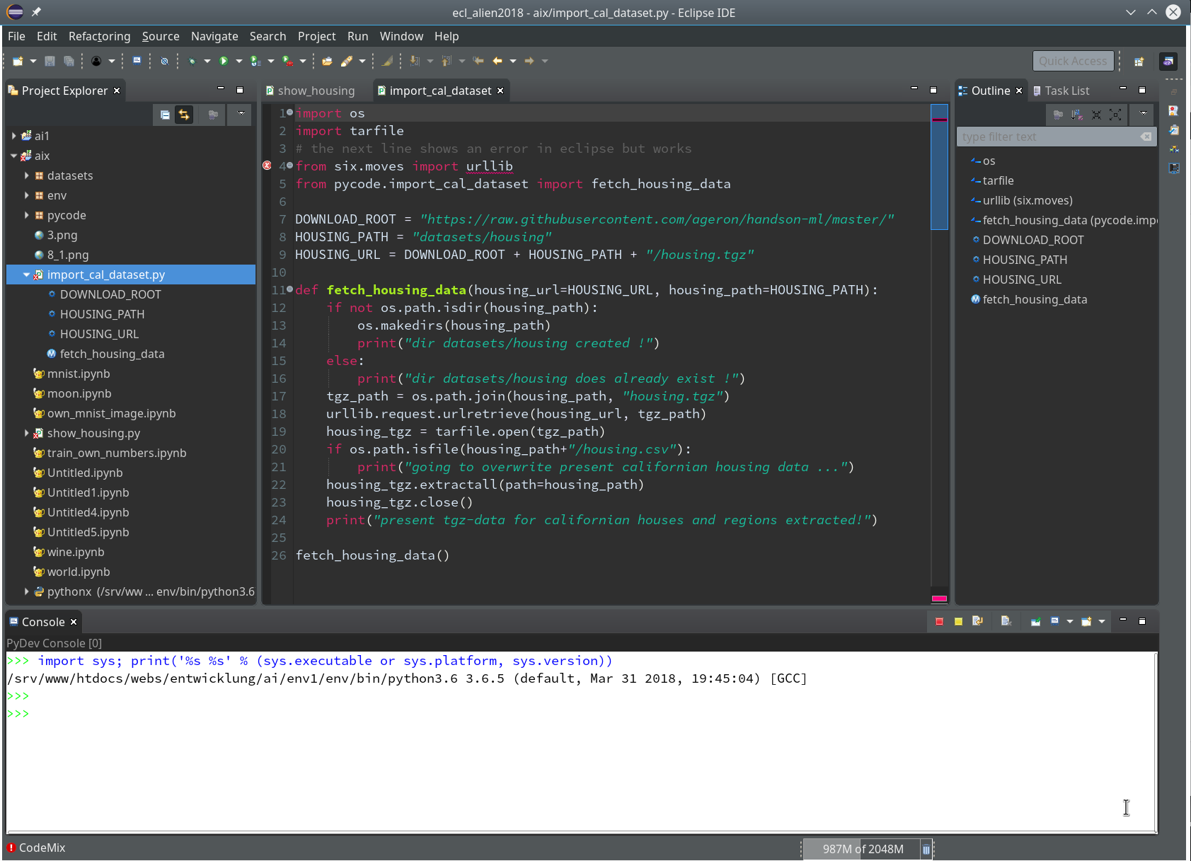
Eventually, you get a full fledged Eclipse IDE interface, which you
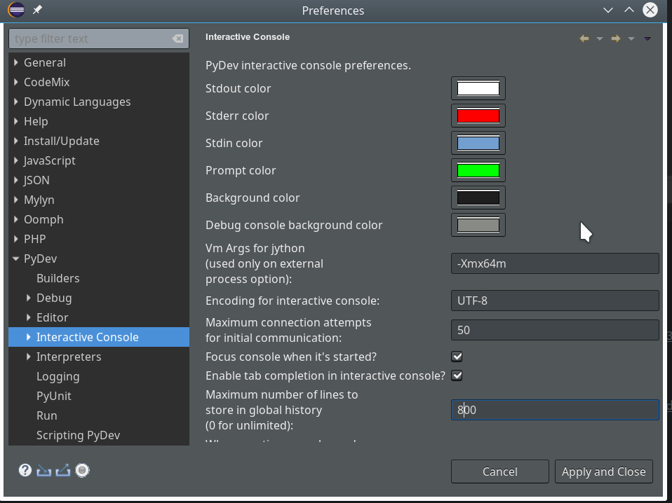
can customize (see “Window >> “Preferences”). This is beyond the scope of this article; I give however some hints regarding color. You can e.g. customize editor and console colors for specific programming languages within Eclipse.
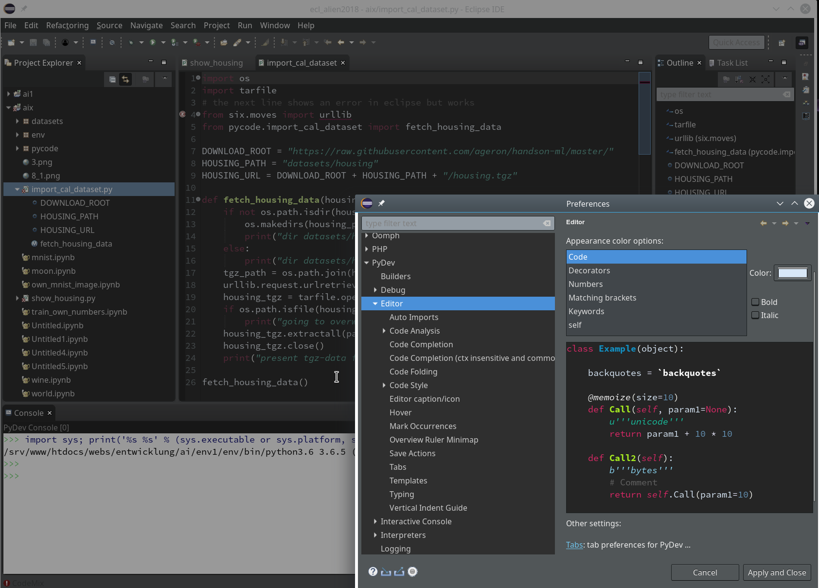
However, regarding certain application control elements you may nevertheless run into trouble regarding the definition of colors; one reason is that on a Qt5-based KDE desktop the end result may depend both on Eclipse settings and also on desktop design schemes for GTK2/GTK3 applications as Eclipse. This type of dependency requires experiments. So, what exactly do I use?
Within Eclipse itself I use the “Dark Theme” – to avoid an eye sore whilst programming.
Regarding my KDE desktop I use a standard Breeze Desktop Scheme with Elegance-Design and the Standard Color Theme (with the activation flag for non-Qt-applications set). KDE application design elements, however, are taken from the Adwaita-Scheme. For GTK2 applications on KDE I prefer the Clearlooks-design, for GTK3 applications – as Eclipse (> 4.9.0) – again Adwaita. This combination gives me a sufficient foreground/background-contrast for control elements like checkboxes, radio buttons, …
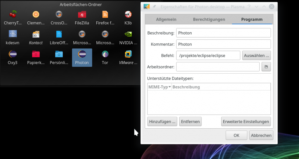
A last convenience point: In a graphical desktop environment as KDE you will of course add some icon to your desktop (in my case with a reference to the file “projects/eclipse/eclipse”) to reduce the starting process to a click.
Step 2: Basic Python packages on the system level
I assume that you have already installed Python in your Linux-(Opensuse)-system. In my environment I use the Python 3.6 RPM-packages from the standard repositories for Opensuse Leap 15.0:
https://download.opensuse.org/distribution/ leap/15.0/repo/oss/
https://download.opensuse.org/update/ leap/15.0/oss/.
The number of available Python library packages is quite big; what libraries you should install depends on your programming objectives. You need at least the basic “python3” package. Another “must”, in my opinion, is the package “python3-pip“; it enables us to perform specific package installations for our “virtual Python environment” later on.
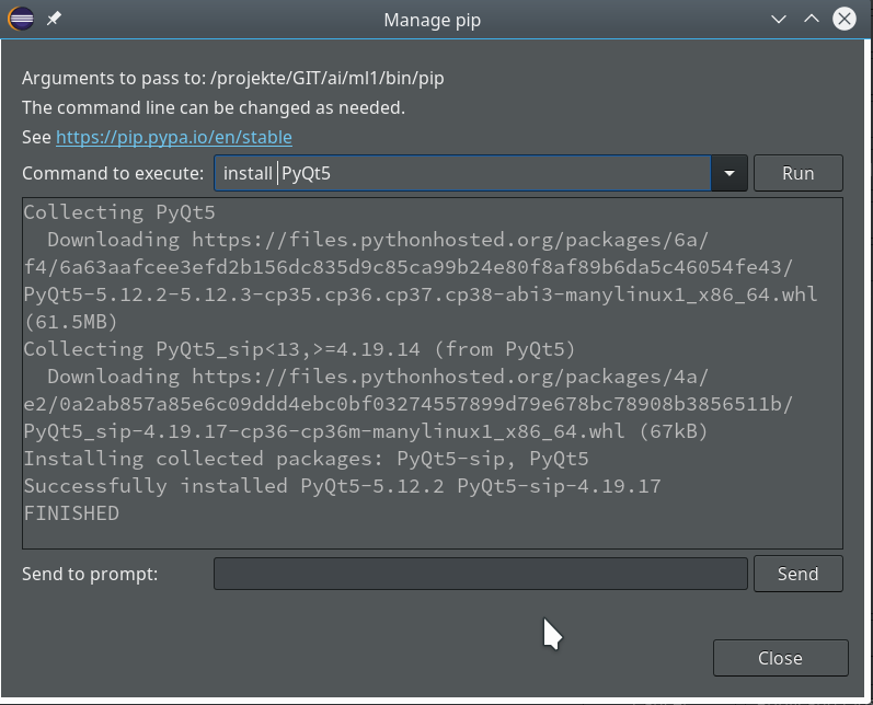
As a basic ingredient for graphics you may also install suitable libraries for your Linux desktop environment. In my case this is KDE – so I installed the packages “python3-qt5″, python-qt5-utils” and also “python3-qt5-devel” to be on the safe side. However, as we shall see we may need Qt5-packages within a project environment, too. That is where Python’s internal “pip” mechanism enters the game.
Below we shall perform the installation of the “virtualenv” package to demonstarte the usage of “pip” or “pip3” in a Python3-environment. As a first step I provide myself (i.e. user “myself”) with a current version of “pip3”:
myself@mytux:~> pip3 --version
pip 19.1.0 from /home/myself/.local/lib/python3.6/site-packages/pip (python 3.6)
myself@mytux:~> pip3 install --user --
upgrade pip
Collecting pip
  Downloading https://files.pythonhosted.org/packages/5c/e0/be401c003291b56efc55aeba6a80ab790d3d4cece2778288d65323009420/pip-19.1.1-py2.py3-none-any.whl (1.4MB)
     |████████████████████████████████| 1.4MB 1.0MB/s
Installing collected packages: pip
  Found existing installation: pip 19.1
    Uninstalling pip-19.1:
      Successfully uninstalled pip-19.1
Successfully installed pip-19.1.1
myself@mytux:~> pip3 --version
pip 19.1.1 from /home/myself/.local/lib/python3.6/site-packages/pip (python 3.6)
You see that the parameter “–user” already lead to a personal configuration of basic Python packages (within my home-directory). But we shall specify a project specific environment in the fourth step.
Step3: Working directory for our ML-project
We now define a base directory “ai” for future experiments.
myself@mytux:~> export AI_PATH ="/projekte/GIT/ai/"
myself@mytux:~> mkdir -p $AI_PATH
A sub-directory “ml1” shall provide the environment for a bunch of initial basic ML-experiments and related Python code files, libraries, Jupyter notebooks, etc.. We create this “ml1” directory as a base for a “virtual” Python environment.
Step 4: Prepare a virtual Python environment via virtualenv and working directories
Python installations allow for the definition of a so called “virtual environment” for projects via the “virtualenv” add-on. Among other things “virtualenv” lets you define a project specific configuration with Python and library versions in a consistent reproducible state. This in turn gives you a base for the “configuration management” of complex endeavors; therefore, I strongly recommend to make use of this feature – also in combination with PyDev: .
myself@mytux:~> pip3 install --user --upgrade virtualenv
Collecting virtualenv
  Downloading https://files.pythonhosted.org/packages/ca/ee/8375c01412abe6ff462ec80970e6bb1c4308724d4366d7519627c98691ab/virtualenv-16.6.0-py2.py3-none-any.whl (2.0MB)
     |████████████████████████████████| 2.0MB 1.6MB/s
Installing collected packages: virtualenv
  Found existing installation: virtualenv 16.5.0
    Uninstalling virtualenv-16.5.0:
      Successfully uninstalled virtualenv-16.5.0
Successfully installed virtualenv-16.6.0
myself@mytux:~> virtualenv --version
16.6.0
myself@mytux:~>
Now we can use “virtualenv” to setup the virtual Python environment for “ml1” in our “ai”-directory:
myself@mytux:~> cd /projekte/GIT/ai/
myself@mytux:/projekte/GIT/ai> virtualenv ml1
Using base prefix '/usr'
  No LICENSE.txt / LICENSE found in source
New python executable in /projekte/GIT/ai/ml1/bin/python3
Also creating executable in /projekte/GIT/ai/ml1/bin/python
Installing setuptools, pip, wheel...
done.
myself@mytux:/projekte/GIT/ai> la ml1
insgesamt 20
drwxr-xr-x 5 myself users 4096 25. Mai 15:05 .
drwxr-xr-x 3 myself users 4096 25. Mai 15:05 ..
drwxr-xr-x 2 myself users 4096 25. Mai 15:05 bin
drwxr-xr-x 2 myself users 4096 25. Mai 15:05 include
drwxr-xr-x 3 myself users 4096 25. Mai 15:05 lib
lrwxrwxrwx 1 myself users    3 25. Mai 15:05 lib64 -> lib
myself@mytux:/projekte/GIT/ai> la ml1/bin
insgesamt 72
drwxr-xr-x 2 myself users  4096 25. Mai 15:05 .
ndrwxr-xr-x 5 myself users  4096 25. Mai 15:05 ..
-rw-r--r-- 1 myself users  2096 25. Mai 15:05 activate
-rw-r--r-- 1 myself users  1428 25. Mai 15:05 activate.csh
-rw-r--r-- 1 myself users  3052 25. Mai 15:05 activate.fish
-rw-r--r-- 1 myself users  1804 25. Mai 15:05 activate.ps1
-rw-r--r-- 1 myself users  1512 25. Mai 15:05 activate_this.py
-rw-r--r-- 1 myself users  1150 25. Mai 15:05 activate.xsh
-rwxr-xr-x 1 myself users   249 25. Mai 15:05 easy_install
-rwxr-xr-x 1 myself users   249 25. Mai 15:05 easy_install-3.6
-rwxr-xr-x 1 myself users   231 25. Mai 15:05 pip
-rwxr-xr-x 1 myself users   231 25. Mai 15:05 pip3
-rwxr-xr-x 1 myself users   231 25. Mai 15:05 pip3.6
lrwxrwxrwx 1 myself users     7 25. Mai 15:05 python -> python3
-rwxr-xr-x 1 myself users 10456 25. Mai 15:05 python3
lrwxrwxrwx 1 myself users     7 25. Mai 15:05 python3.6 -> python3
-rwxr-xr-x 1 myself users  2338 25. Mai 15:05 python-config
-rwxr-xr-x 1 myself users   227 25. Mai 15:05 wheel
myself@mytux:/projekte/GIT/ai>
You see that a whole directory structure was established – with Python3 executables copied from our basic system installation. We can fully use this Python environment already on the command line (of a terminal window). However, we need to activate it so that its files and libs are really used:
myself@mytux:/projekte/GIT/ai/ml1> source bin/activate
(ml1) myself@mytux:/projekte/GIT/ai/ml1> python3
Python 3.6.5 (default, Mar 31 2018, 19:45:04) [GCC] on linux
Type "help", "copyright", "credits" or "license" for more information.
>>> print("Hello World!")
Hello World!
>>> quit()
(ml1) myself@mytux:/projekte/GIT/ai/ml1> pip3 install --upgrade jupyter
Collecting jupyter
  Using cached https://files.pythonhosted.org/packages/83/df/0f5dd132200728a86190397e1ea87cd76244e42d39ec5e88efd25b2abd7e/jupyter-1.0.0-py2.py3-none-any.whl
Collecting notebook (from jupyter)
...
..Successfully built pyrsistent
Installing collected packages: Send2Trash, ipython-genutils, decorator, six, traitlets, jupyter-core, MarkupSafe, jinja2, pyzmq, python-dateutil, tornado, jupyter-client, backcall, pickleshare, wcwidth, prompt-toolkit, ptyprocess, pexpect, pygments, parso, jedi, ipython, ipykernel, prometheus-client, pyrsistent, attrs, jsonschema, nbformat, terminado, entrypoints, mistune, webencodings, bleach, testpath, defusedxml, pandocfilters, nbconvert, notebook, jupyter-console, widgetsnbextension, ipywidgets, qtconsole, jupyter
Successfully installed MarkupSafe-1.1.1 Send2Trash-1.5.0 attrs-19.1.0 backcall-0.1.0 bleach-3.1.0 decorator-4.4.0 defusedxml-0.6.0 entrypoints-0.3 ipykernel-5.1.1 ipython-7.5.0 ipython-genutils-0.2.0 ipywidgets-7.4.2 jedi-0.13.3 jinja2-2.10.1 jsonschema-3.0.1 jupyter-1.0.0 jupyter-client-5.2.4 jupyter-console-6.0.0 jupyter-core-4.4.0 mistune-0.8.4 nbconvert-5.5.0 nbformat-4.4.0 notebook-5.7.8 pandocfilters-1.4.2 parso-0.4.0 pexpect-4.7.0 pickleshare-0.7.5 prometheus-client-0.6.0 prompt-toolkit-2.0.9 ptyprocess-0.6.0 pygments-2.4.1 pyrsistent-0.15.2 python-dateutil-2.8.0 pyzmq-18.0.1 qtconsole-4.5.0 six-1.12.0 terminado-0.8.2 testpath-0.4.2 tornado-6.0.2 traitlets-4.3.2 wcwidth-0.1.7 webencodings-0.5.1 widgetsnbextension-3.4.2
(ml1) myself@mytux:/projekte/GIT/ai/ml1/include> cd ../bin
(ml1) myself@mytux:/projekte/GIT/ai/ml1/bin> la
insgesamt 152
drwxr-xr-x 2 myself users  4096 26. Mai 14:22 .
drwxr-xr-x 7 myself users  4096 26. Mai 14:22 ..
-rw-r--r-- 1 myself users  2096 25. Mai 15:05 activate
-rw-r--r-- 1 myself users  1428 25. Mai 15:05 activate.csh
-rw-r--r-- 1 myself users  3052 25. Mai 15:05 activate.fish
n-rw-r--r-- 1 myself users  1804 25. Mai 15:05 activate.ps1
-rw-r--r-- 1 myself users  1512 25. Mai 15:05 activate_this.py
-rw-r--r-- 1 myself users  1150 25. Mai 15:05 activate.xsh
-rwxr-xr-x 1 myself users   249 25. Mai 15:05 easy_install
-rwxr-xr-x 1 myself users   249 25. Mai 15:05 easy_install-3.6
-rwxr-xr-x 1 myself users   250 26. Mai 14:22 iptest
-rwxr-xr-x 1 myself users   250 26. Mai 14:22 iptest3
-rwxr-xr-x 1 myself users   243 26. Mai 14:22 ipython
-rwxr-xr-x 1 myself users   243 26. Mai 14:22 ipython3
-rwxr-xr-x 1 myself users   232 26. Mai 14:22 jsonschema
-rwxr-xr-x 1 myself users   238 26. Mai 14:22 jupyter
-rwxr-xr-x 1 myself users   252 26. Mai 14:22 jupyter-bundlerextension
-rwxr-xr-x 1 myself users   237 26. Mai 14:22 jupyter-console
-rwxr-xr-x 1 myself users   242 26. Mai 14:22 jupyter-kernel
-rwxr-xr-x 1 myself users   280 26. Mai 14:22 jupyter-kernelspec
-rwxr-xr-x 1 myself users   238 26. Mai 14:22 jupyter-migrate
-rwxr-xr-x 1 myself users   240 26. Mai 14:22 jupyter-nbconvert
-rwxr-xr-x 1 myself users   239 26. Mai 14:22 jupyter-nbextension
-rwxr-xr-x 1 myself users   238 26. Mai 14:22 jupyter-notebook
-rwxr-xr-x 1 myself users   240 26. Mai 14:22 jupyter-qtconsole
-rwxr-xr-x 1 myself users   259 26. Mai 14:22 jupyter-run
-rwxr-xr-x 1 myself users   243 26. Mai 14:22 jupyter-serverextension
-rwxr-xr-x 1 myself users   243 26. Mai 14:22 jupyter-troubleshoot
-rwxr-xr-x 1 myself users   271 26. Mai 14:22 jupyter-trust
-rwxr-xr-x 1 myself users   231 25. Mai 15:05 pip
-rwxr-xr-x 1 myself users   231 25. Mai 15:05 pip3
-rwxr-xr-x 1 myself users   231 25. Mai 15:05 pip3.6
-rwxr-xr-x 1 myself users   234 26. Mai 14:22 pygmentize
lrwxrwxrwx 1 myself users     7 25. Mai 15:05 python -> python3
-rwxr-xr-x 1 myself users 10456 25. Mai 15:05 python3
lrwxrwxrwx 1 myself users     7 25. Mai 15:05 python3.6 -> python3
-rwxr-xr-x 1 myself users  2338 25. Mai 15:05 python-config
-rwxr-xr-x 1 myself users   227 25. Mai 15:05 wheel
Looking into the lib-directory is also informative. I leave this to the user.
(ml1) myself@mytux:/projekte/GIT/ai/ml1/bin> cd ../lib/python3.6/site-package
(ml1) myself@mytux:/projekte/GIT/ai/ml1/lib/python3.6/site-packages> la
Step 5: Install some important libraries for ML studies
As we are occupied with installing packages, let us get some more packages typically required to do experiments for AI/ML:
(ml1) myself@mytux:/projekte/GIT/ai/ml1> pip3 install --upgrade matplotlib numpy pandas scipy scikit-learn
....
Step 6: Install PyDev for Eclipse
The previous steps were all on the level of the Linux-system and/or for a special Python environment for me as a user. But Eclipse does not know anything about Python, yet. We need a special Python environment within Eclipse with suitable editors, project and test environments, configuration options and so on for our Python based machine learning projects.
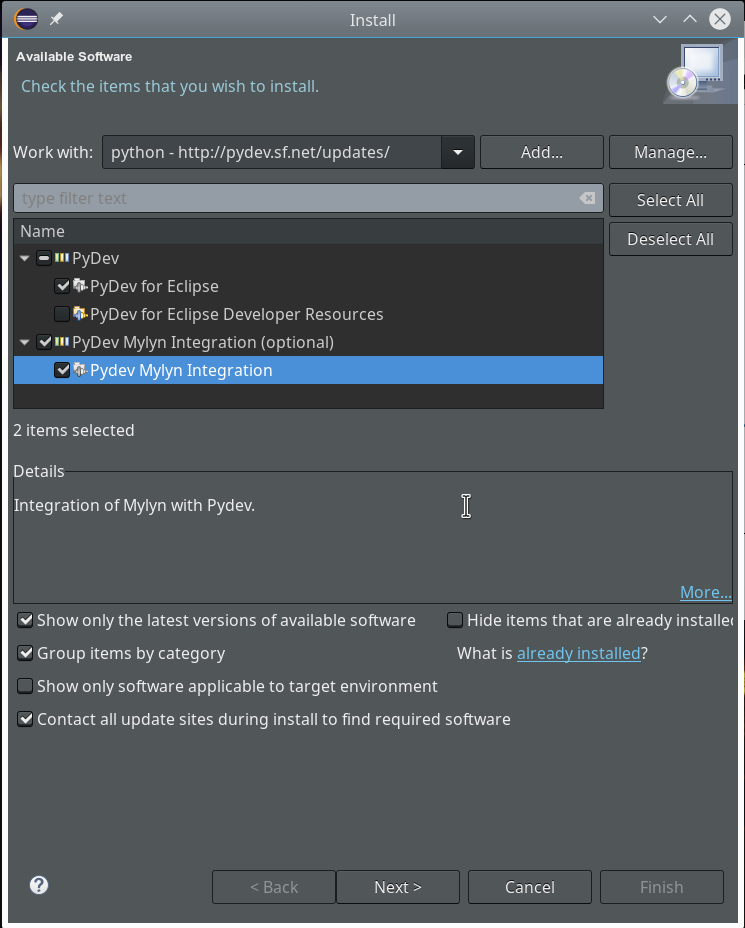
You find the necessary PyDev plugins for Eclipse at the site http://pydev.sf.net/updates/.
The easiest way to install PyDev is: Add this site to the update configuration of Eclipse – via the menu point “Help >> Install new software”. Click the “Add”-Button there. In the popup you provide a name for the site and its URL. Then you choose this site “to work with” and click on the relevant plugin “PyDev for Eclipse”. If you are a fan of Mylyn you also load the respective package.
Step 7: Change to a PyDev perspective within Eclipse
After having installed the PyDev packages we can start Eclipse and change
the layout by choosing a Python specific “perspective“.
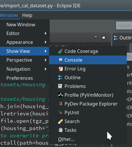
We start with the menu point
“Window >> Perspective >> Open Perspective >> Other …”
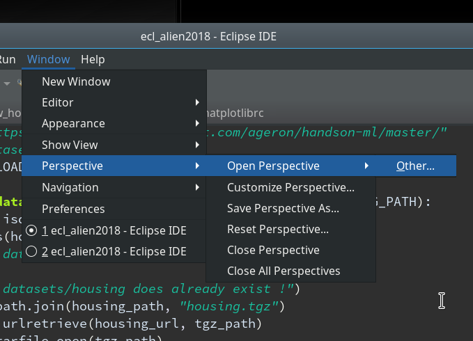
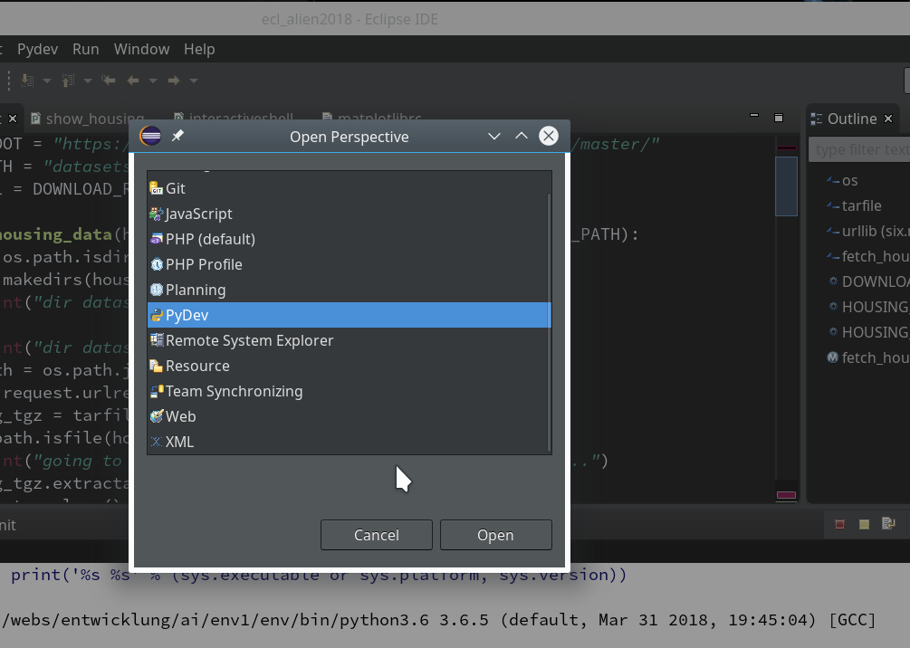
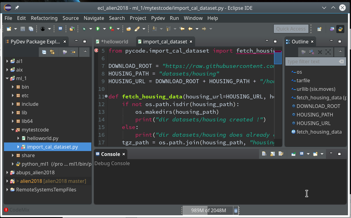
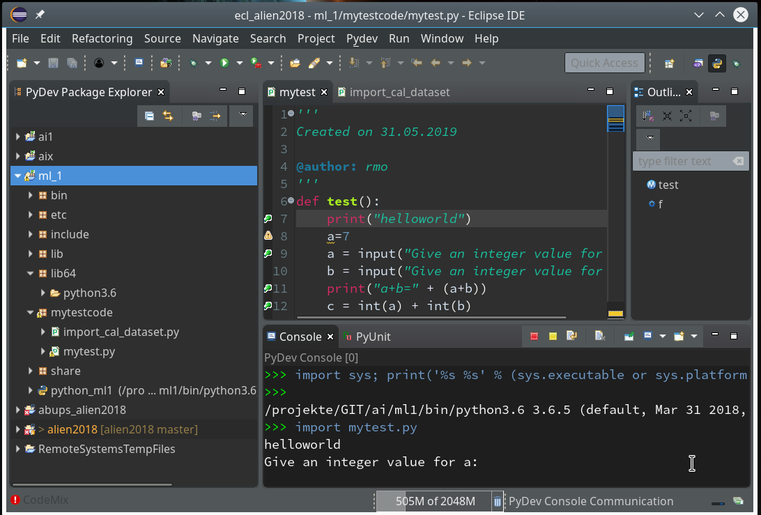
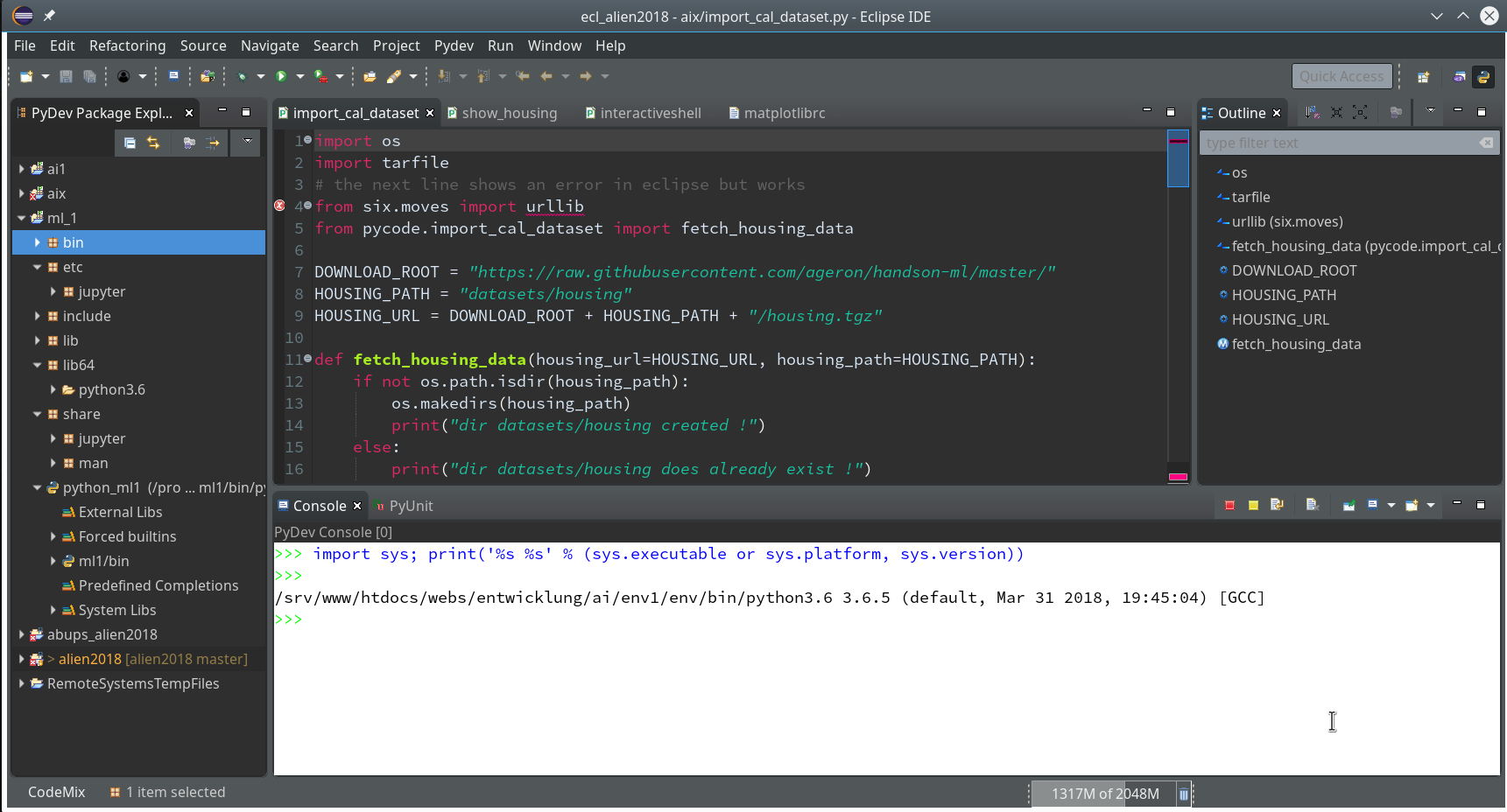
Then we choose “PyDev” and end up with the a layout of Eclipse similar to the following (you may have some other position arrangements of the sub-windows):
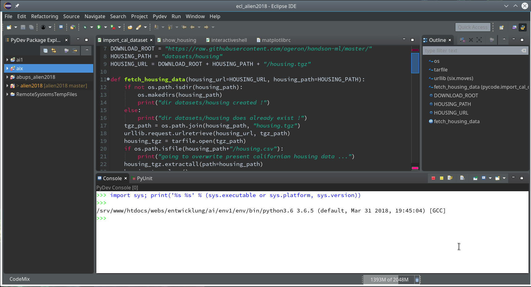
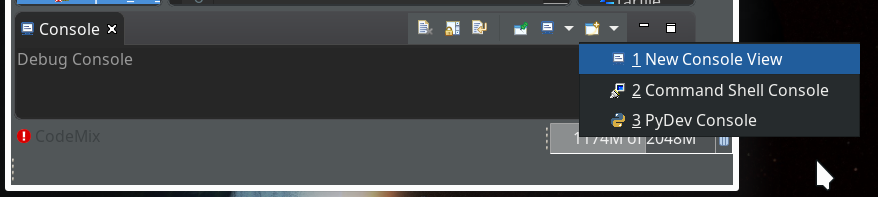
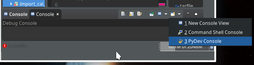
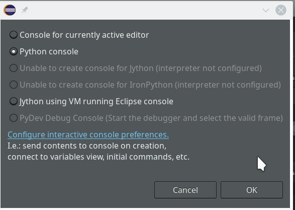
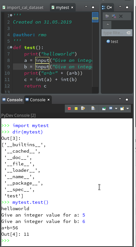
On the left side you see some projects, which I had set up already. (As I integrate some of my Python experiments with PHP-programs the reader may detect some PHP-projects, too …). In the lower right part of the IDE we see a console view for interactive python commands. I come back to this point below.
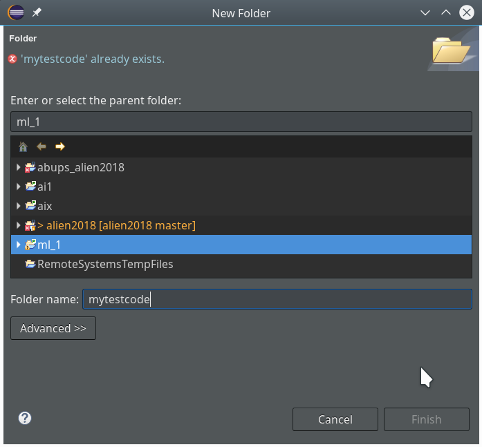
Step 8: Add a Python project in Eclipse for our virtual environment ml1
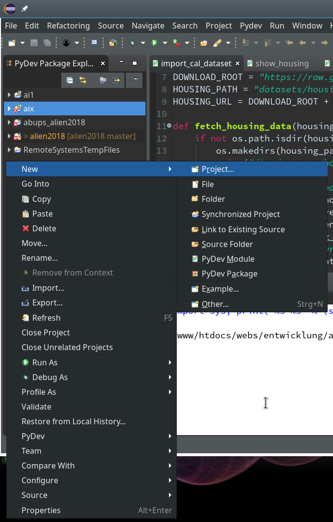
We now create a new project which shall be related to our directory “/projekte/GIT/ai/ml1”. A right mouse click into the leftmost area gives us:
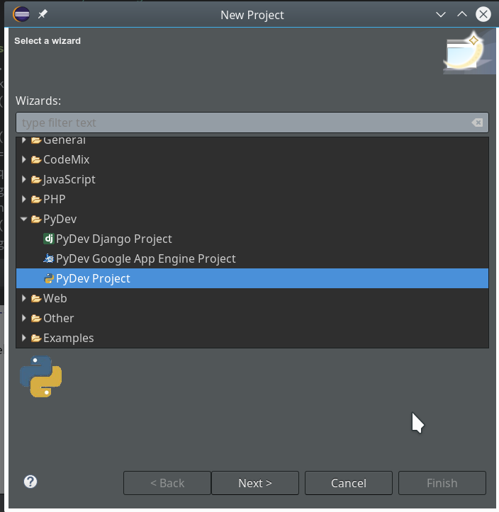
On the next popup we choose a “PyDev”-project type.
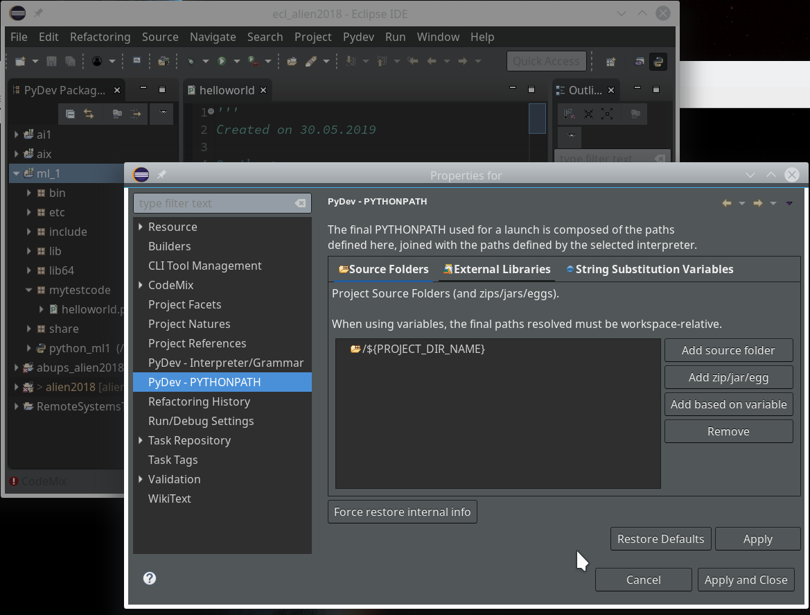
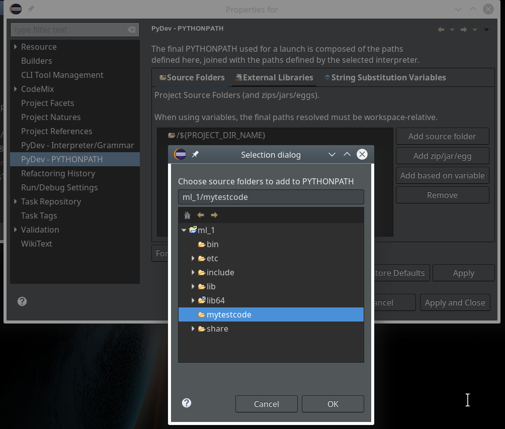
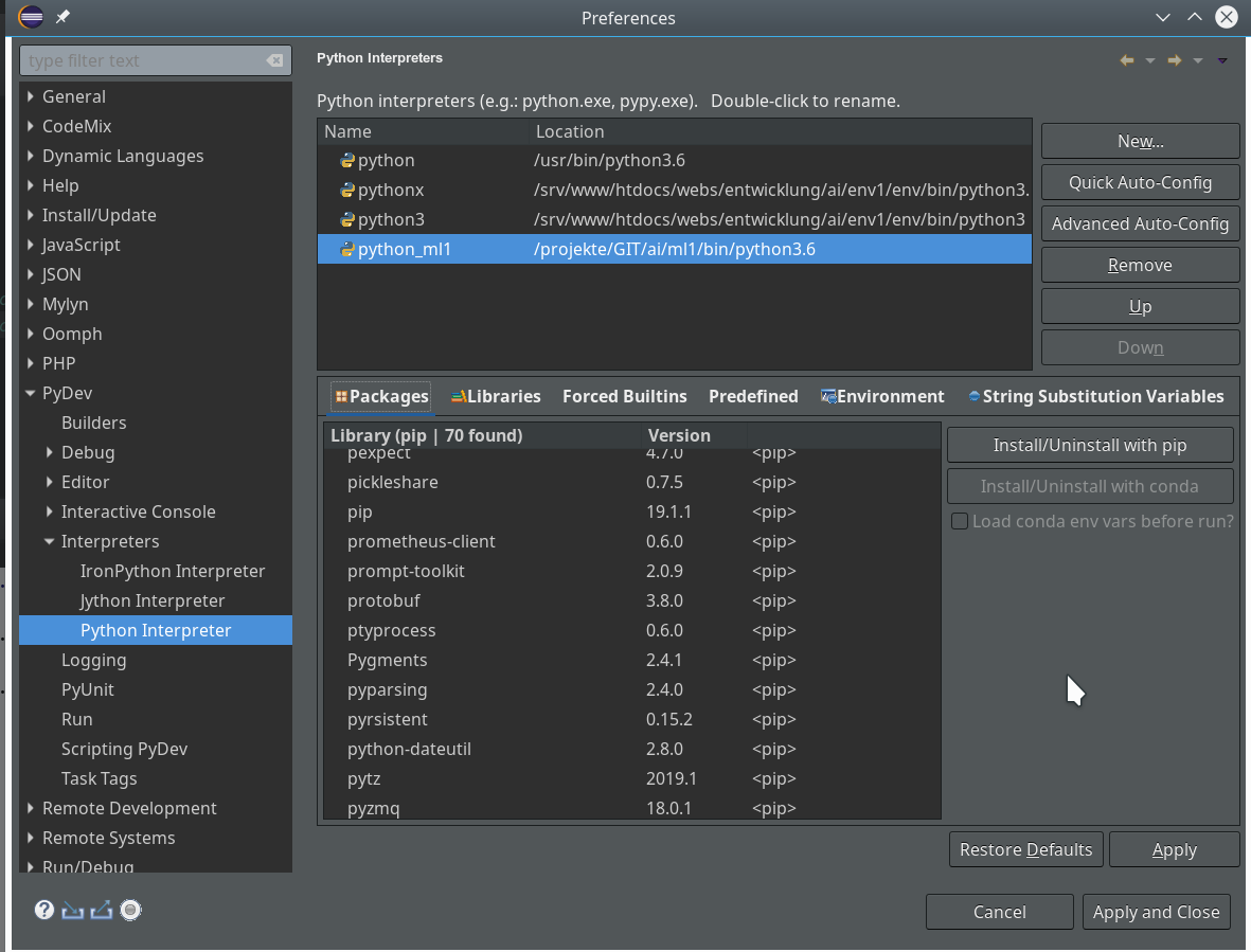
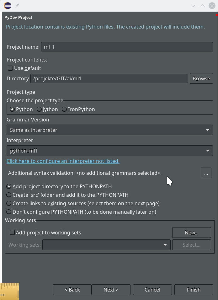
On the third screen we first enter our path “/projekte/GIT/ai/ml1” – with this setting we see all the modules and libraries loaded for our virtual environment in Eclipse, too.
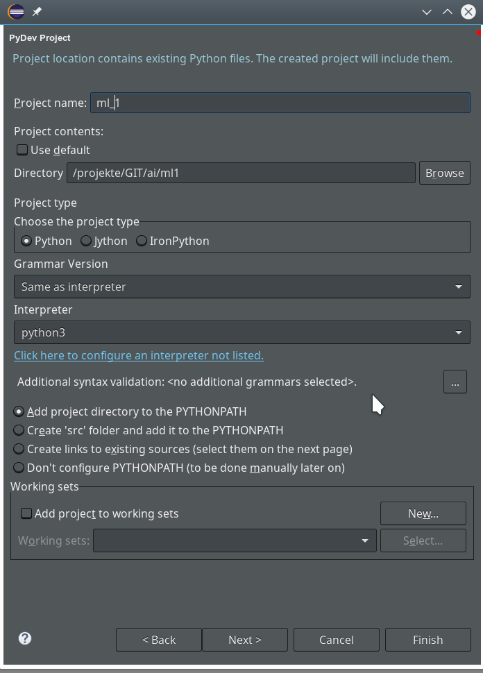
The important interpreter setting – it decides on the usage of our virtualenv
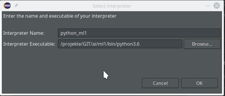
Really interesting is the field for the choice of an “Interpreter“. Here we get the option to refer to our “virtual environment”. When we click on the blue link we can configure an interpreter and related path settings. On the opening popup window we enter the path to the interpreter of our ml1-environment, i.e. to “/projekte/GIT/ai/ml1/bin/python3.6“.
We go on and get
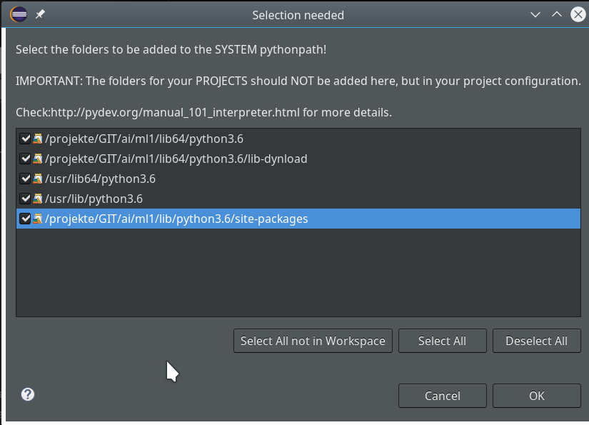
Important: We do not delete the references to the systems libraries here!
We move on and come back to our project definition window – we now
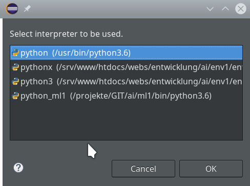
choose the interpreter “python_ml1” which we defined a minute ago.
On the next screen we do not yet have any other projects to be referenced.
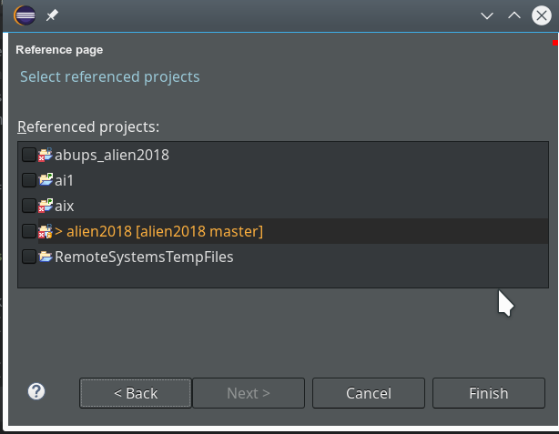
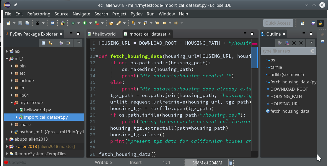
So we finish and get our first Python3 project:
Enough for today. In the second article
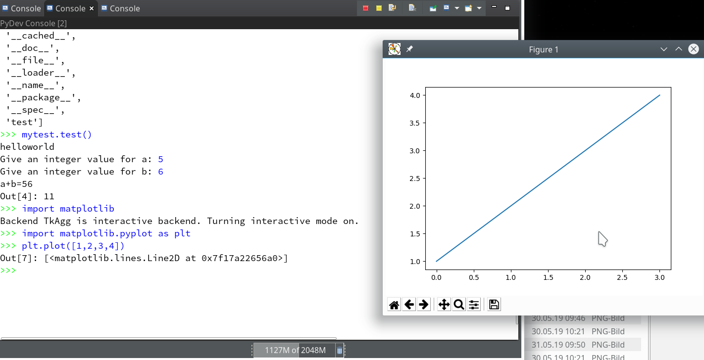
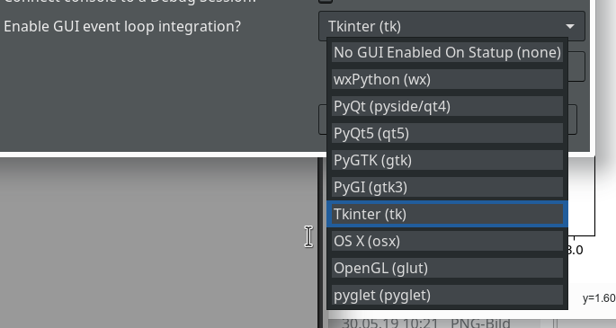
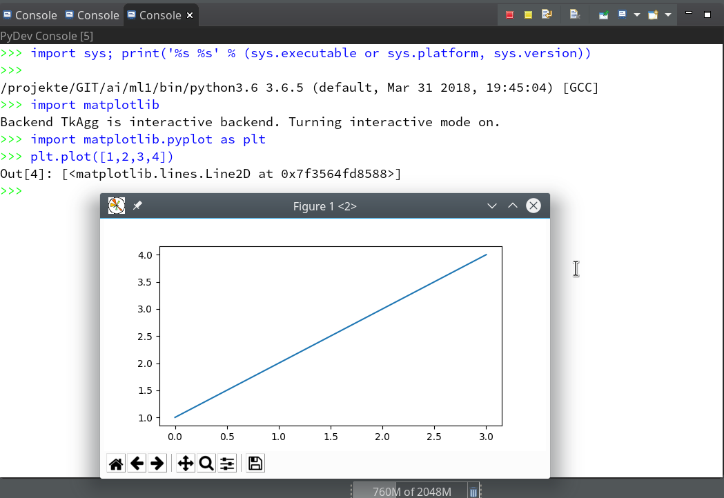
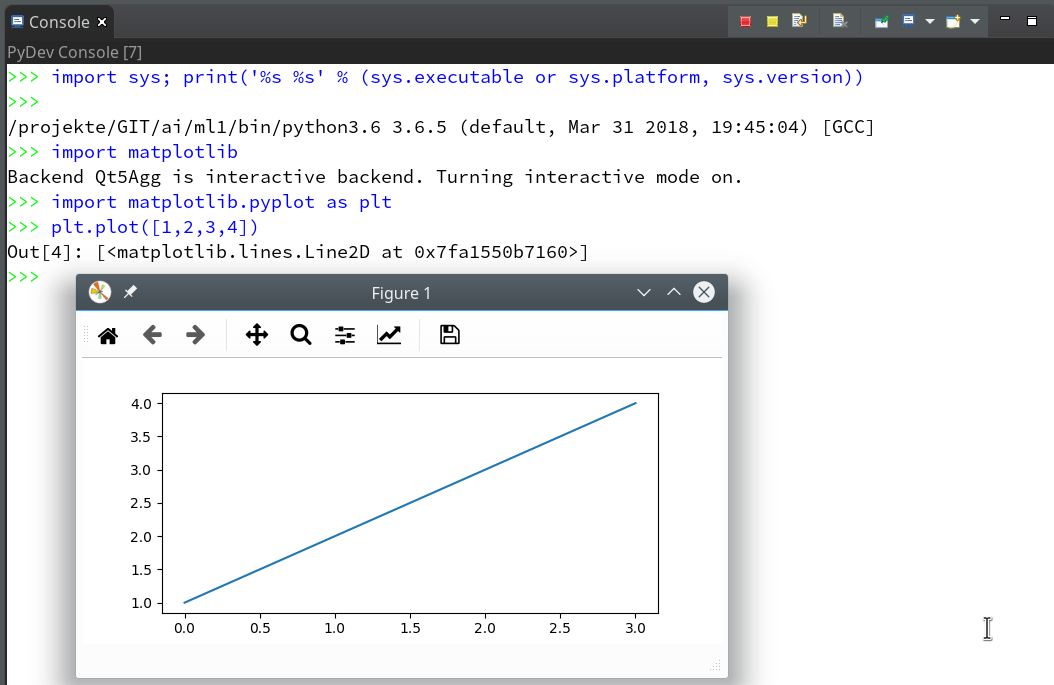
Eclipse, PyDev, virtualenv and graphical output of matplotlib on KDE – II
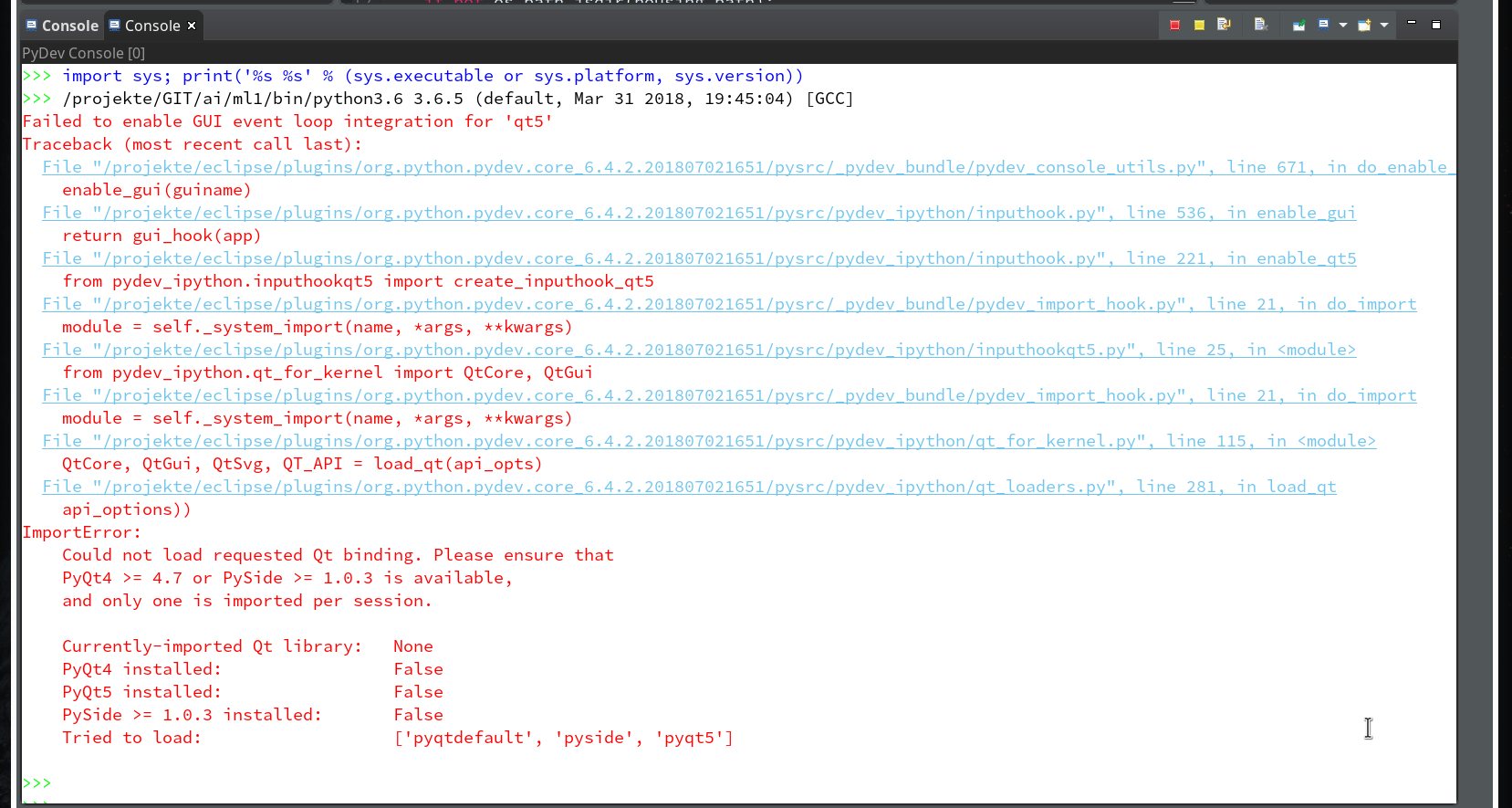
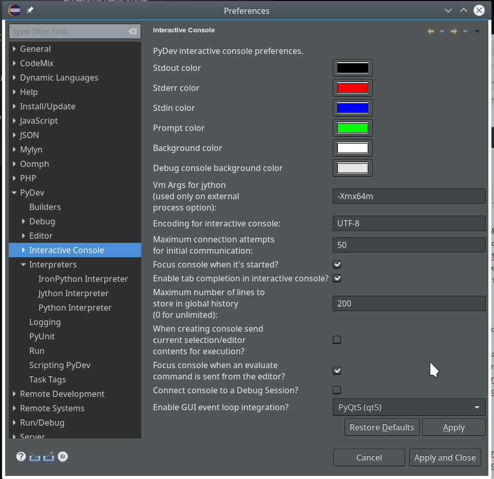
of this series we shall use a Python-console within Eclipse for interactive coding and the display of results. We shall see that we need additional settings to get matplotlib to work.
Stay tuned …
Links
https://www.caktusgroup.com/blog/2011/08/31/getting-started-using-python-eclipse/