This post requires Javascript to display formulas!
Convolutional Autoencoders and multivariate normal distributions
Experiments as with my own on convolutional Autoencoders [CAE] show: A CAE maps a training set of human face images (e.g. CelebA) onto an approximate multivariate vector distribution in the CAE’s latent space Z. Each image corresponds to a point (z-point) and a corresponding vector (z-vector) in the CAE’s multidimensional latent space. More precisely the results of numerical experiments showed:
The multidimensional density function which describes the inner dense core of the z-point distribution (containing more than 80% of all points) was (aside of normalization factors) equivalent to the density function of a multivariate normal distribution [MND] for the respective z-vectors in an Euclidean coordinate system.
For results of my numerical CAE-experiments see
Autoencoders and latent space fragmentation – X – a method to create suitable latent vectors for the generation of human face images
and related previous posts in this blog. After the removal of some outliers beyond a high sigma-level (≥ 3) of the original distribution the remaining core distribution fulfilled conditions of standard tests for multivariate normal distributions like the Shapiro-Wilk test or the Henze-Zirkler test.
After a normalization with an appropriate factor the continuous density functions controlling the multivariate vector distribution can be interpreted as a probability density function [p.d.f.]. The components vj (j=1, 2,…, n) of the vectors to the z-points are regarded as logically separate, but not uncorrelated variables. For each of these variables a component specific value distribution Vj is given. All these marginal distributions contribute to a random vector distribution V, in our case with the properties of a MND:
\]
μ is a vector with all mean values μj of the Vj component distributions as its components. Σ abbreviates the covariance matrix relating the distributions Vj with one another.
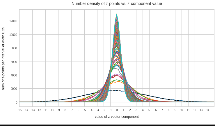
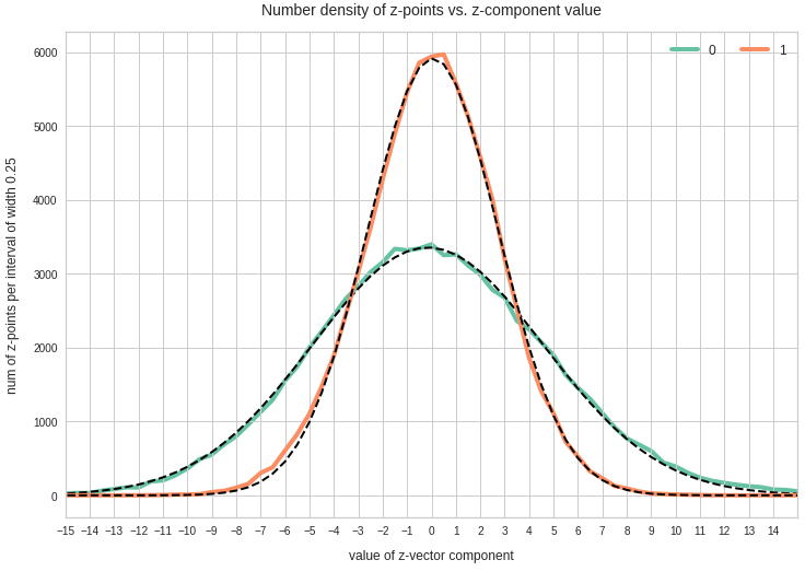
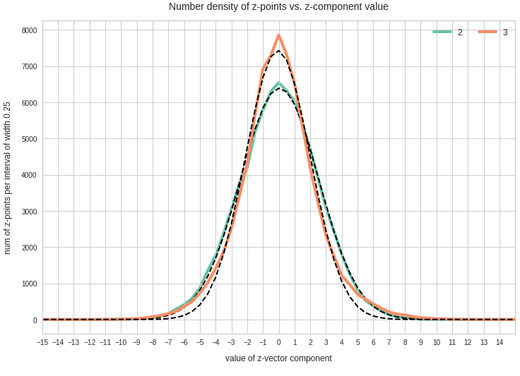
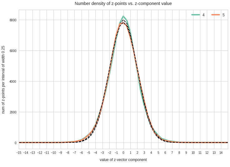
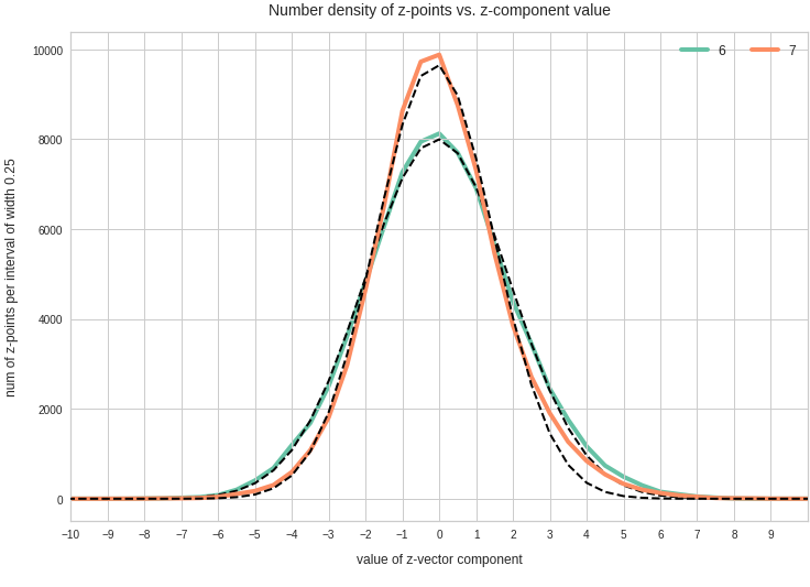
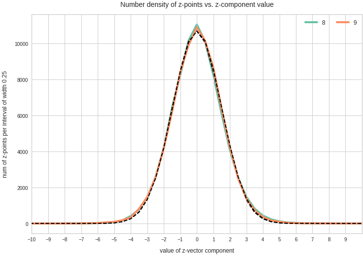
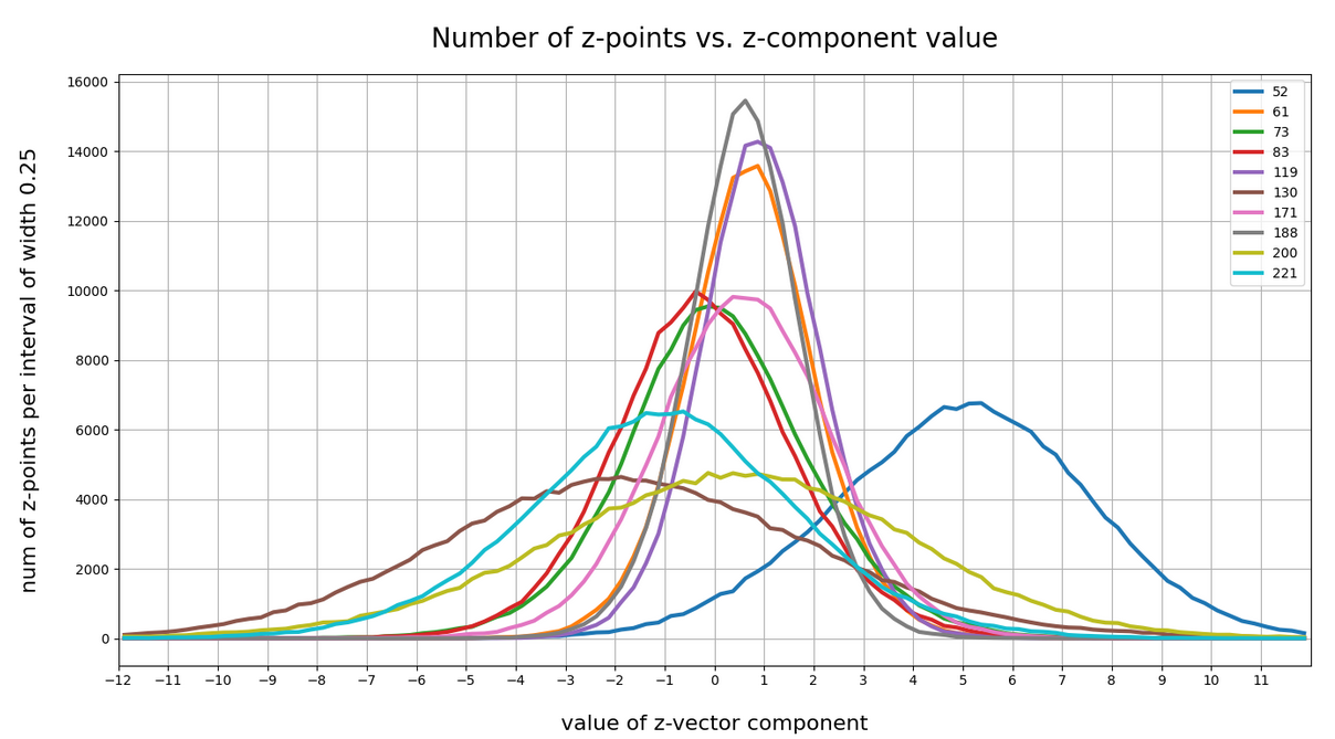
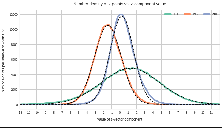
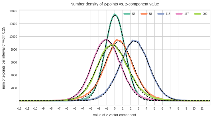
The point distribution of a CAE’s MND forms a complex rotated multidimensional ellipsoid with its center somewhere off the origin in the latent space. The latent space itself typically has many dimensions. In the case of my numerical experiments the number of dimension was n ≥ 256. The number of sample vectors used were between 80,000 and 200,000 – enough data to approximate the vector distribution by a continuous density function. The densities for the Vj-distributions formed a smooth Gaussian function (for a reasonable sampling interval). But note: One has to be careful: The fact that the Vj have a Gaussian form is not a sufficient condition for a MND. (See the next post.) But if a MND is given all Vj have a Gaussian form.
Generative use of MNDs in multidimensional latent spaces of high dimensionality
When we want to use a CAE as a generative tool we need to solve a problem: We must create statistical vectors which point into the (multidimensional) volume of our point distribution in the latent space of the encoding algorithm. Only such vectors provide useful information to the Decoder of the CAE. A full multivariate normal distribution and hyperplanes of its multidimensional density function are difficult to analyze and to control when developing a proper numerical algorithm. Therefore I want to reduce the problem of vector generation to a sequence of viewable and controllable 2-dimensional problems. How can this be achieved?
A central property of a multivariate normal distribution helps: Any sub-selection of m vector-component distributions forms a multivariate normal distribution, too (see below). For m=2 and for vector components indexed by (j,k) with respective distributions Vj, Vk we get a so called “bivariate normal distribution” [BND]:
\]
A MND has n*(n-1)/2 such subordinate BNDs. The 2-dim density function of a bivariate normal distribution
\]
for vector component values vj, vk defines a point density of the sample data in the (j,k)-coordinate plane of the Euclidean coordinate system in which the MND is described. The density function of the marginal distributions Vj showed the typical Gaussian forms of a univariate normal distribution.
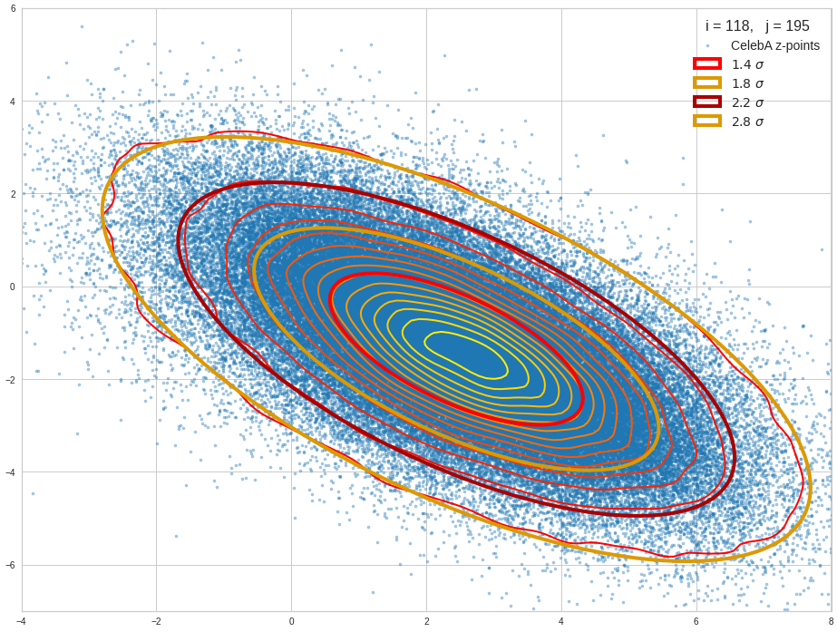
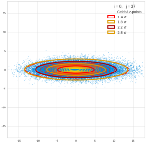
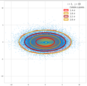
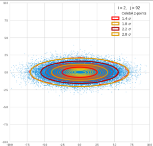
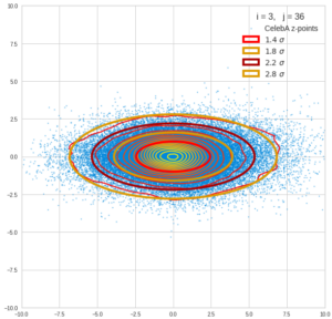
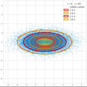
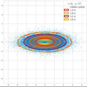
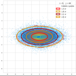
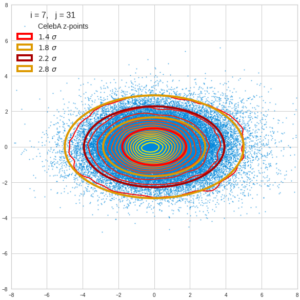
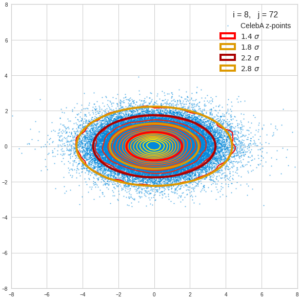
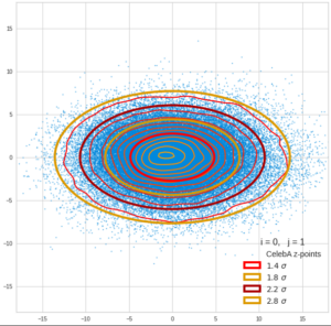
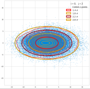
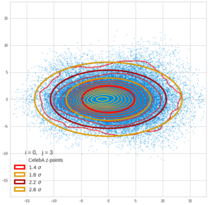
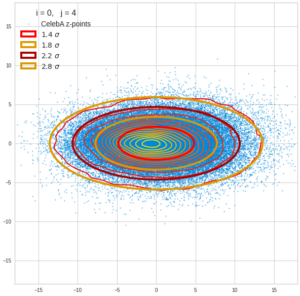
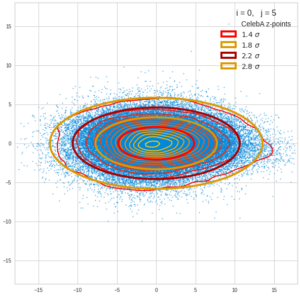
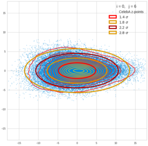
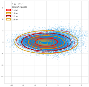
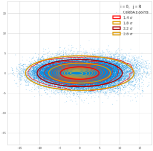
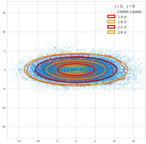
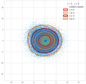
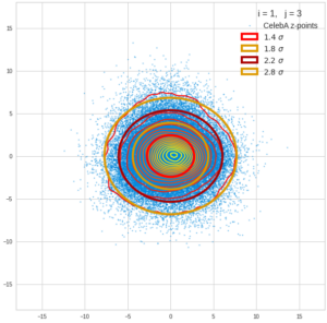
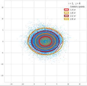
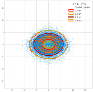
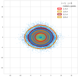
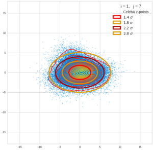
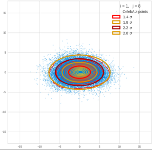
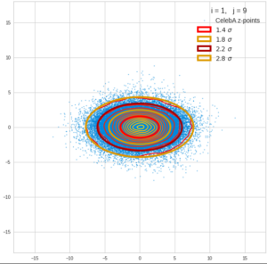
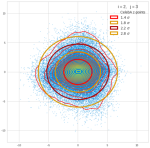
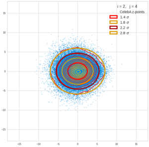
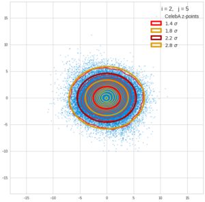
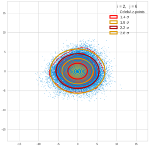
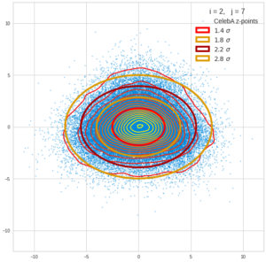
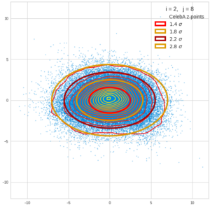
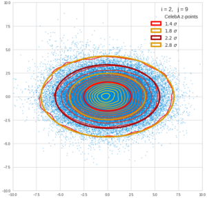
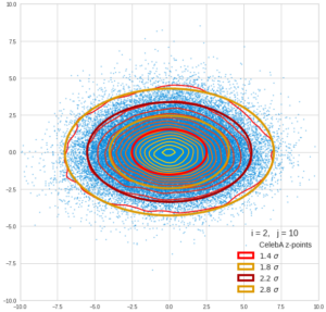
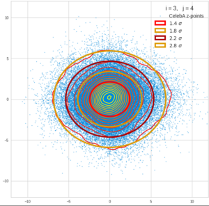
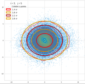
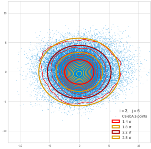
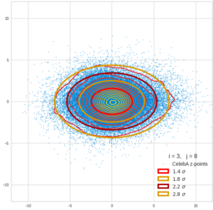
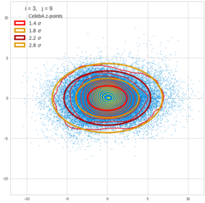
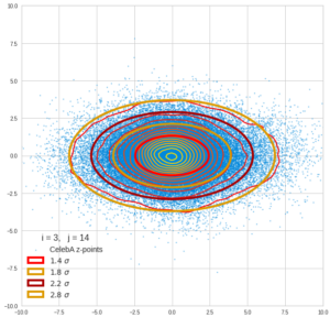
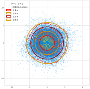
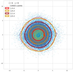
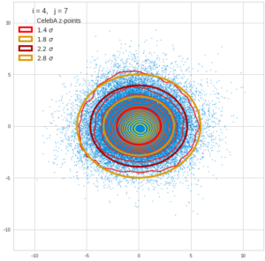
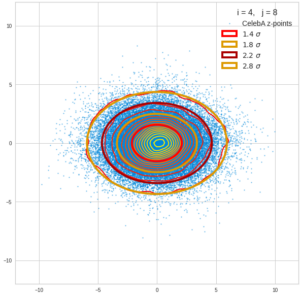
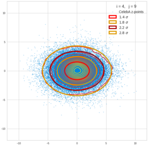
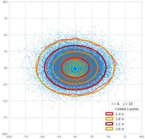
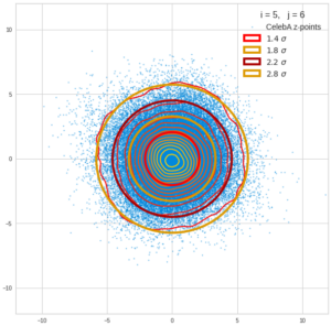
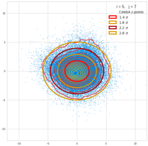
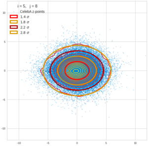
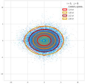
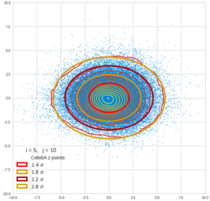
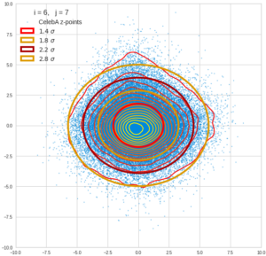
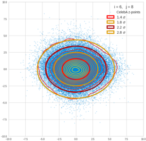
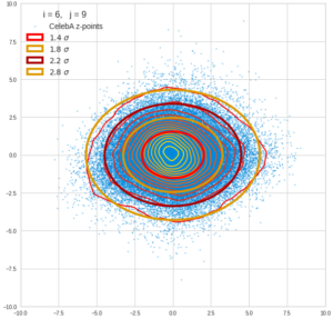
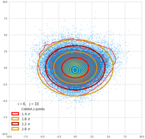
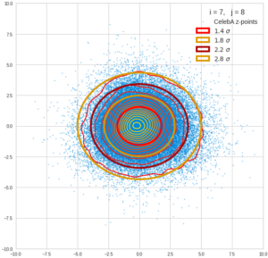
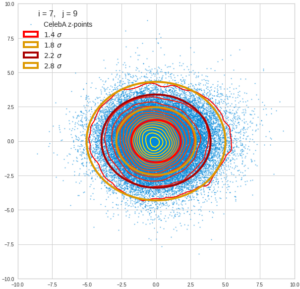
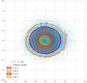
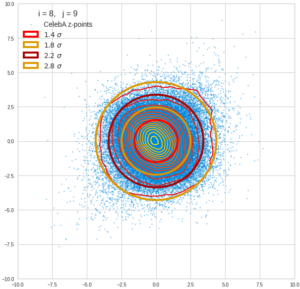
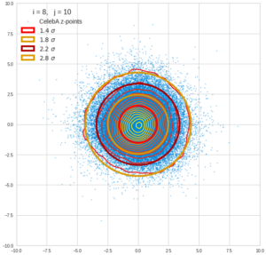
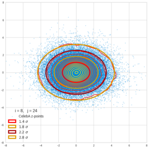
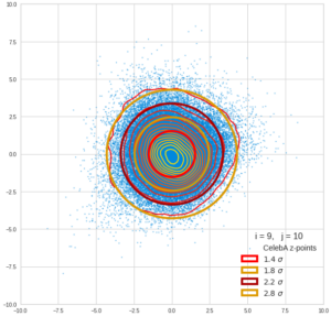
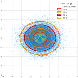
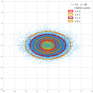
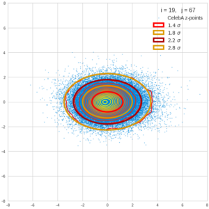
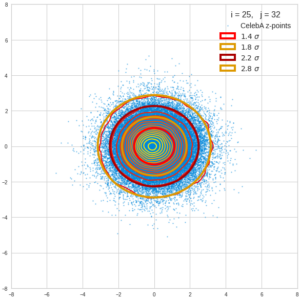
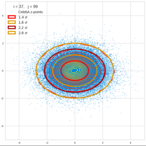
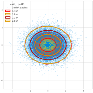
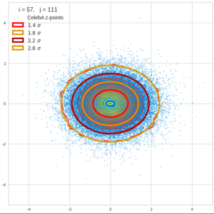
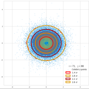
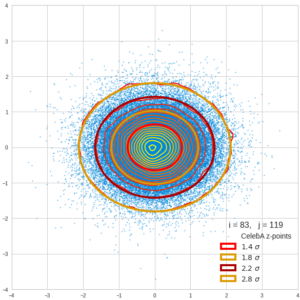
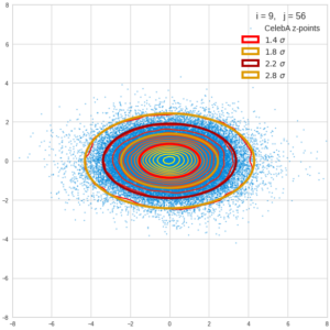
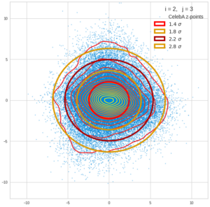
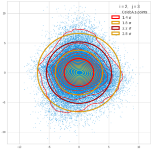
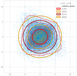
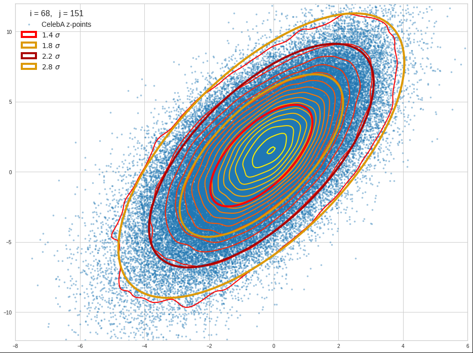
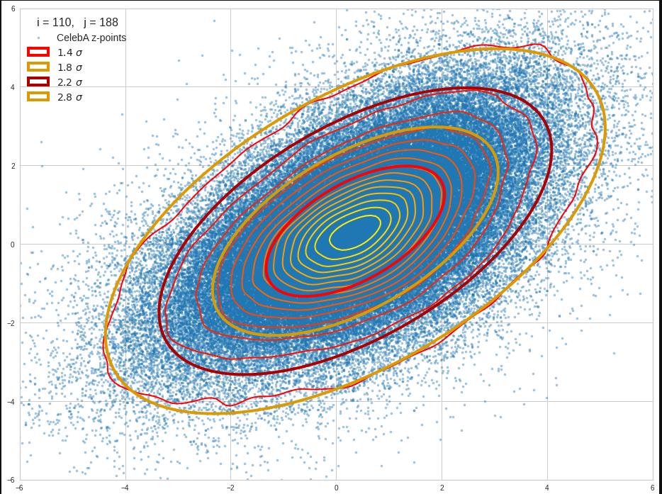
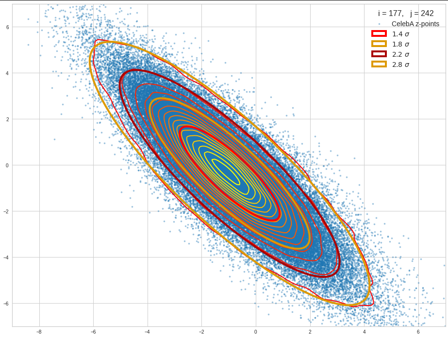
The density function of a BND has some interesting mathematical properties. Among other things: The hyperplanes of constant density of a BND’s density function form ellipses. This is illustrated by the following plots showing such contour lines for selected pairs (Vj, Vk) of a real point-distribution in a 256-dimensional latent space. The point distribution was created by a CAE in its latent space for the CelebA dataset.
Contour lines for selected (j,k)-pairs. The thick lines stem from theory and calculated correlation coefficients of the univariate distributions.
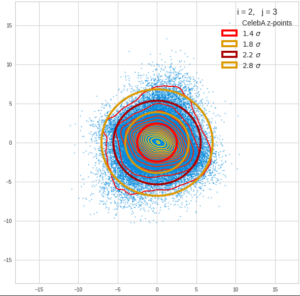
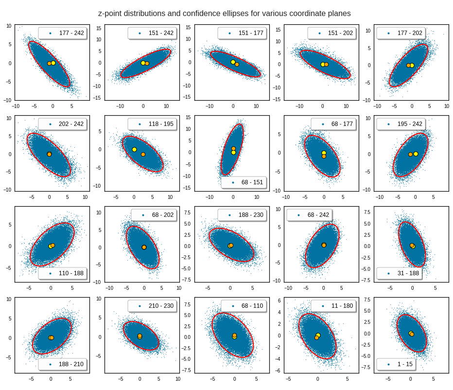
The next plot shows the contours of selected vector-component pairs after a PCA-transformation of the full MND. (Main ellipse axes are now aligned with the axes of the PCA-coordinate system):

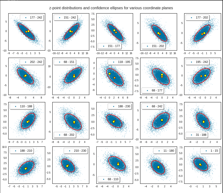
These ellipses with axes along the coordinate axes are relatively easy to handle. They can be used for vector creation. But they require a full PCA transformation of the MND-distribution, a PCA-analysis for complexity reduction and an application of the inverse PCA-transformation. The plot below shows the point-density compared to a 2.2-σ-confidence ellipses. The orange points are the results of a proper statistical numerical vector generation algorithm based on a PCA-transformation of the MND.
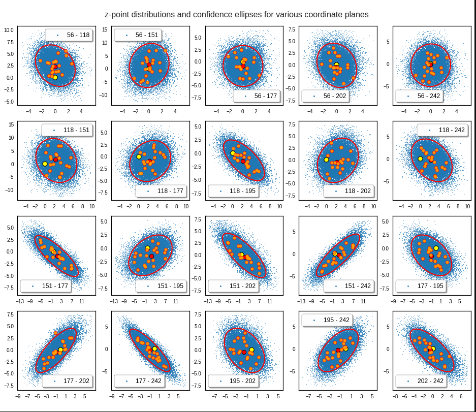
See my post quoted above for the application of a PCA-transformation of the multidimensional MND for vector creation.
However, we get the impression that we could also use these rotated ellipses in projections of the MND onto coordinate planes of the original latent space system directly to impose limiting conditions on the component values of statistical vectors pointing to an inner regions of the MND. Of course, a generated statistical vector must then comply with the conditions of all such ellipses. This requires an analysis and combined use of the ellipses of all of the subordinate BNDs of a the original MND during an iterative or successive definition of the values for the vector components.
Objective of this post series
In my last post about CAEs (see the link given above) I have explicitly asked the question whether one can avoid performing a full PCA-transformation of the MND when creating statistical vectors pointing to a defined inner region of a MND.
The objective of this post series is to prove the answer: Yes, we can. And we will use the BNDs resulting from projections of the original MND onto coordinate planes. We will in particular explore the n*(n-1)/2 the properties of the BNDs’ confidence ellipses. As said: These ellipses are rotated against the coordinate system’s axes. We will have to deal with this in detail. We will also use properties of their 1-dimensional marginal distributions (projections onto the coordinate axes, i.e. the Vj.)
In addition we need to prepare a variety of formulas before we are able to define numerical procedure for the vector generation without a full PCA-transformation of the MND with around 100,000 vectors. Some of the derived formulas will also allow for a deeper insight into how the multiple BNDs of a MND are related between each other and with confidence hypersurfaces of the MND.
Ellipses in general lead to equations governed by quadratic or fourth power polynomials. We will in addition use some elementary correlation formula from statistics and for some exercises a simple optimization via derivatives. The series can be regarded as an excursion into some of the math which governs bivariate distributions resulting from a MND.
As MNDs may also be the result of other generative Machine Learning algorithms in respective latent spaces, the whole approach to statistical vector generation for such cases should be of general interest. Note also that the so called “central limit theorem” almost guarantees the appearance of MNDs in many multivariate datasets with sufficiently large samples and value dependencies on many singular observations.
Distributions of a variety of variables may result in a MND if the variables themselves depend on many individual observables with limited covariance values of their distributions. In particular pairwise linearly correlated Gaussian density distributions individual variables (seen as vector components) may constitute a MND if the conditional probabilities fulfill some rules. We will see a glimpse of this in 2 dimensions when we analyze integrals over Gaussians in the bivariate normal case.
Other approaches to statistical vector generation?
Well, we could try to reconstruct the multidimensional density function of the MND. This is a challenge which appears in some problems of pure statistics, but also in experimental physics. See e.g. a paper of Rafey Anwar, Madeline Hamilton, Pavel M. Nadolsky (2019, Department of Physics, Southern Methodist University, Dallas; https://arxiv.org/pdf/1901.05511.pdf). Then we would have to find the elements of the (inverse) covariance matrix or – equivalently – the elements of a multidimensional rotation matrix. But the most efficient algorithms to get the matrix coefficients again work with projections onto coordinate planes. I prefer to use properties of the ellipses of the bivariate distributions directly.
Note that using the multidimensional density function of the MND directly is not of much help if we want to keep the vectors’ end points within a defined multidimensional inner region of the distribution. E.g.: You want to limit the vectors to some confidence region of the MND, i.e. to keep them inside a certain multidimensional ellipsoidal contour hyper-surface. The BND-ellipses in the coordinate planes reflect the multidimensional ellipsoidally shaped contour hyperplanes of the full distribution. Actually, when we vertically project a multidimensional hyperplane onto a coordinate plane then the outer 2-dim border line coincides with a contour ellipse of the respective BND. (This is due to properties of a MND. We will come back to this in a future post.) The problem of proper limiting individual vector component values thus again is best solved by analyzing properties of the BNDs.
Steps, methods, mathematical level
As a first step I will, for the sake of completeness, write down the formula for a multivariate normal distribution, discuss a bit its mathematical construction from uncorrelated univariate normal distribution. I will also list up some basic properties of a MND (without proof!). These properties will justify our approach to create statistical vectors pointing into a defined inner region of the MND by investigating projected contour ellipses of all subordinate BNDs. As a special aspect I want to make it at least plausible, why the projected contour ellipses define infinitesimal regions of the same relative probability level as their multidimensional counterparts – namely the multidimensional ellipsoidal hypersurfaces which were projected onto coordinate planes.
Then as a first productive step I want to motivate the specific mathematical form of the probability density function [p.d.f] of a bivariate normal distribution. In contrast to many of the math papers I have read on the topic I want to use a symmetry argument to derive the basic form of the p.d.f. I will point out an important, but plausible assumption about conditional distributions. An analogous assumption on the multidimensional level is central for the properties of a MND.
As the distributions Vj and Vk can be correlated we then want to understand the impact of the correlation coefficients on the parameters of the 2-dimensional density function. To achieve this I will again derive the density function by using our previous central assumption and some simple relations between the expectation values of the constituting two univariate distributions in the linear correlation regime. This concludes the part of the series where we get familiar with BNDs.
Furthermore we are interested in features and consequences of the 2-dimensional density functions. The contour lines of the 2-dim density function are ellipses – rotated by some specific angle. I will look at a formal mathematical process to construct such ellipses – in particular confidence ellipses. I will refer to the results Carsten Schelp has provided in an Internet article on this topic.
His construction process starts with a basic ellipse, which I will call base correlation ellipse [BCE]. The length of the axes of this ellipse are eigenvalues of the covariance matrix of the standardized marginal distributions constituting the BND. The main axes of this elementary ellipse are in addition aligned with the two selected axes of a basic Euclidean coordinate system in which the bivariate distribution is defined. The length of the BCE’s main axes can be shown to depend on the correlation coefficient for the two vector component distributions Vj and Vk. This coefficient also appears in the precision matrix of the BND. Points on the base correlation ellipse can be mapped with two steps of an affine transformation onto points on the real contour ellipses, in particular to points of the confidence ellipses.
The whole construction process is not only of immense help when designing visualization programs for the contour ellipses of our distribution with many (around 100,000) individual vectors. The process itself gives us some direct geometrical insights. It also helps to avoid finding a numerical solution of the usual eigenvector-problems when answering some specific questions about the rotated contour ellipses. Normally we solve an eigenvalue-problem for the covariance matrix of the multi- or the many subordinate bi-variate distributions to get precise information about contour ellipses. This corresponds to a transformation of the distributions to a new coordinate system whose axes are aligned to the main axes of the ellipses. Numerically this transformation is directly related to a PCA transformation of the vector distributions. However, such a PCA-transformation can be costly in terms of CPU time.
Instead, we only need a numerical determination of all the mutual the correlation coefficients of the univariate marginal distributions of the MND. Then the eigenvalue problem on the BND-level is already analytically solved. We therefore neither perform a full numerical PCA analysis of the MND and multidimensional rotation of the vectors of around 100,000 samples. Nor do we analyze explained variance ratios to determine the most important PCA components for dimensionality reduction. We neither need to perform a numerical PCA analysis of the BNDs.
Most important: Our problem of vector generation is formulated in the original latent space coordinate system and it gets a direct solution there. The nice thing is that Schelp’s construction mechanism reduces the math to the solution of quadratic polynomial equations for the BNDs. The solutions of those equations, which are required for our ultimate purpose of vector generation, can be stated in an explicit form.
Therefore, the math in this series will mostly remain on high school level (at least at a level given when I was young). Actually, it was fun to dive back into exercises reminding me of school 50 years ago. I hope the interested reader has some fun, too.
Solutions to some particular problems with respect to the confidence ellipses of the MND’s BNDs
In particular we will solve the following problems:
- Problem 1: The two points on the BCE-ellipse with the same vj-value are not mapped onto points with the same vj-value on the confidence ellipse. We therefore derive the coordinates of points on the BCE-ellipse that give us one and the same vj-value on the real confidence ellipse.
- Problem 2: Plots for a real MND vector distribution indicate that all (n-1) confidence ellipses of distribution pairs of a common Vj with other marginal distributions Vk (for the same confidence level and with k ≠ j) have a common tangent parallel to one coordinate axis. We will derive the value of a maximum v_j-value for all ellipses of (j,k)-pairs of vector component distributions. We will prove that it is identical for all k. This will define the common interval of allowed vj-component-values for a bunch of confidence ellipses for all (Vj, Vk)-pairs with a common Vj.
- Problem 3: The BCE-ellipses for a common j-, but different k-values depend on different values for the correlation coefficients ρj,k of Vj with its various Vk counterparts. Therefore we need a formula that relates a point on the BCE-ellipse leading to a concrete v_j-value of the mapped point on the confidence ellipse of a particular (Vj, Vk)-pair to respective points on other BCE-ellipses of different (Vj, Vm)-pair with the same resulting v_j-value on their confidence ellipses. I will derive such a formula. It will help us to apply multiple conditions onto the vector component values.
- Problem 4: As a supplemental exercise we will derive a mathematical expression for the size of the main axes and the rotation angle of the ellipses. We should, of course, get values that are identical to results of the eigenwert-problem for the correlation matrix (describing a PCA coordinate transformation). This gives us additional confidence in Schelps’ approach.
In the end we can use our results to define a numerical algorithm for the direct creation of vectors pointing to a defined inner region of the multivariate normal distribution. As said, this algorithms does not require a costly PCA transformations of the full MND or many, namely n*(n-1)/2 such PCA-transformations of its BNDs.
I intend to visualize all results with the help of a concrete example of a multivariate example distribution created by a CAE for the CelebA dataset. The plots will use Schelp’s construction algorithm for the confidence ellipses extensively.
Conclusion and outlook
Convolutional Autoencoders create approximate multivariate normal distributions [MND] for certain input data (with Gaussian pattern properties) in their latent space. MNDs appear in other contexts of machine learning and statistics, too. For evaluation and generative purposes one may need statistical vectors with end points inside a defined multidimensional hypersurface corresponding to a certain confidence level and a certain constant density value of the MND’s density function. These hypersurfaces are multidimensional ellipsoids.
We have the hope that we can use mathematical properties of the MND’s subordinate bivariate normal distributions [BNDs] to create statistical vectors with end points inside the multidimensional confidence ellipsoids of a MND. Typically such an ellipsoid resides off the origin of the latent space’s coordinate system and the ellipsoid’s main axes are rotated against the axes of the coordinate system. We intend to base the confining conditions on the components of the aspired statistical vectors on correlation coefficients of the marginal vector component distributions. Our numerical algorithm should avoid a full PCA-transformation of the multidimensional vector distribution.
In the next post of this series I give a formula for the density function of a multivariate normal distribution. In addition I will list up some basic properties which justify the vector generation approach via bivariate normal distributions.

