
In the last posts of this series
Variational Autoencoder with Tensorflow – I – some basics
Variational Autoencoder with Tensorflow – II – an Autoencoder with binary-crossentropy loss
I have discussed basics of Autoencoders. We have also set up a simple Autoencoder with the help of the functional Keras interface to Tensorflow 2. This worked flawlessly and we could apply our Autoencoder [AE] to the MNIST dataset. Thus we got a good reference point for further experiments. Now let us turn to the design of “Variational Autoencoders” [VAEs].
In the present post I want to demonstrate that some simple classical recipes for the construction of VAEs may not work with Tensorflow [TF] > version 2.3 due to “eager execution mode”, which is activated as the default environment for all command interpretation and execution. This includes gradient determination during the forward pass through the layers of an artificial neural network [ANN]. In contrast to “graph mode” for TF 1.x versions.
Addendum 25.05.2022: This post had to be changed as its original version contained wrong statements.
As we know already form the first post of this series we need a special loss function to control the parameters of distributions in the latent space. These distributions are used to calculate z-points for individual samples and must be “fit” optimally. I list four methods to calculate such a loss. All methods are taken form introductory books on Machine Learning (see the book references in the last section of this post). I use one concrete and exemplary method to realize a VAE: We first extend the layers of the AE-Encoder by two layers (“mu”, “var_log”) which give us the basis for the calculation of z-points on a statistical distribution. Then we use a special layer on top of the Decoder model to calculate the so called “Kullback-Leibler loss” based on data of the “mu” and “var_log” layers. Our VAE Keras model will be based on the Encoder, the Decoder and the special layer. This approach will give us a typical error message to think about.
Building a VAE
A VAE (as an AE) maps points/vectors of the “variable space” to points/vectors in the low-dimensional “latent space”. However, a VAE does not calculate the “z-points” directly. Instead it uses a statistical variable distribution around a mean value. This opens up for further degrees of freedom, which become subjects to the optimization process. These degrees of freedom are a mean value “mu” of a distribution and a “standard deviation”. The latter is derived from a variance “var“, of which we take the logarithm “log_var” for practical and numerical reasons.
Note: Our neural network parts of the VAE will decide themselves during training for which samples they use which mu and which var_log values. They optimize the required values via specific weights at special layers.
A special function
We first define a function whose meaning will become clear in a minute:
# Function to calculate a z-point based on a Gaussian standard distribution
def sampling(args):
    mu, log_var = args
    # A randomized value from a standard distribution
    epsilon = B.random_normal(shape=B.shape(mu), mean=0., stddev=1.)
    # A point in a Gaussian standard distribution defined by mu and var with log_var = log(var)
    return mu + B.exp(log_var / 2) * epsilon
This function will be used to calculate z-points from other variables, namely mu and log_var, of the Encoder.
The Encoder
The VAE Encoder looks almost the same as the Encoder of the AE which we build in the last post:
z_dim = 16

# The Encoder
# ************
encoder_input = Input(shape=(28,28,1))
x = encoder_input
x = Conv2D(filters = 32, kernel_size = 3, strides = 1, padding='same')(x)
x = LeakyReLU()(x)
x = Conv2D(filters = 64, kernel_size = 3, strides = 2, padding='same')(x)
x = LeakyReLU()(x)
x = Conv2D(filters = 128, kernel_size = 3, strides = 2, padding='same')(x)
x = LeakyReLU()(x)

# some information we later need for the decoder - for MNIST and our layers (7, 7, 128)
shape_before_flattening = B.int_shape(x)[1:]  # B is the tensorflow.keras backend ! See last post.

x = Flatten()(x)of

# differences to AE-models. The following layers central elements of VAEs!
mu      = Dense(z_dim, name='mu')(x)
log_var = Dense(z_dim, name='log_var')(x)

# We calculate z-points/vectors in the latent space by a special function
# used by a Keras Lambda layer
enc_out = Lambda(sampling, name='enc_out_z')([mu, log_var])

# The Encoder model
encoder = Model(encoder_input, [enc_out], name="encoder")
encoder.summary()
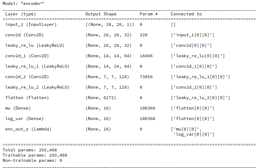
The differences to the AE of the last post comprise two extra Dense layers: mu and log_var. Note that the dimension of the respective rank 1 tensor (a vector!) is equal to z_dim.
mu and log_var are (vector) variables which later shall be optimized. So, we have to treat them as trainable network variables. In the above code this is done via the weights of the two defined Dense layers which we integrated in the network. But note that we did not define any activation function for the layers! The calculation of “output” of these layers is done in a more complex function which we encapsulated in the function “sampling()”.
of
Therefore, we have in addition defined a Lambda layer which applies the (Lambda) function “sampling()” to the vectors mu and var_log. The Lambda layer thus delivers the required z-point (i.e. a vector) for each sample in the z-dimensional latent space.
z-point calculation
How exactly do we calculate a z-point or vector in the latent space? And what does the KL loss, which we later shall use, punish? For details you need to read the literature. But in short terms:
Instead of calculating a z-point directly we use a Gaussian distribution depending on 2 parameters – our mean value “mu” and a standard deviation “var“. We calculate a statistically random z-point within the range of this distribution. Note that we talk about a vector-distribution. The distribution “variables” mu and log_var are therefore vectors.
If “x” is the last layer of our conventional network part then
mu = Dense(self.z_dim, name='mu')(x)
log_var = Dense(self.z_dim, name='log_var')(x)
Having a value for mu and log_var we use a randomized factor “epsilon” to calculate a “variational” z-point with some statistical fluctuation:
epsilon = B.random_normal(shape=B.shape(mu), mean=0., stddev=1.)
z_point = mu + B.exp(log_var/2)*epsilon
This is the core of the “sampling()”-function which we defined a minute ago, already.
As you see the randomization of epsilon assumes a standard Gaussian distribution of possible values around a mean = 0 with a standard-deviation of 1. The calculated z-point is then placed in the vicinity of a fictitious z-point “mu”. The coordinate of mu” and the later value for log_var are subjects of optimization. More specifically, the distance of mu to the center of the latent space and too big values of the standard-deviation around mu will be punished by the loss. Mathematically this is achieved by the KL loss (see below). It will help to get a compact arrangements of the z-points for the training samples in the z-space (= latent space).
To transform the result of the above calculation into an ordinary z-point output of the Encoder for a given input sample we apply a Keras Lambda layer which takes the mu- and log_var-layers as input and applies the function “sampling()“, which we have already defined, to input in form of the mu and var_log tensors.
The Decoder
The Decoder is pretty much the same as the on which we have defined earlier for the Autoencoder.
dec_inp_z = Input(shape=(z_dim))
x = Dense(np.prod(shape_before_flattening))(dec_inp_z)
x = Reshape(shape_before_flattening)(x)
x = Conv2DTranspose(filters=64, kernel_size=3, strides=2, padding='same')(x)
x = LeakyReLU()(x)
x = Conv2DTranspose(filters=32, kernel_size=3, strides=2, padding='same')(x)
x = LeakyReLU()(x)
x = Conv2DTranspose(filters=1,  kernel_size=3, strides=1, padding='same')(x)
x = LeakyReLU()(x)
# Output -
x = Activation('sigmoid')(x)
dec_out = x
decoder = Model([dec_inp_z], [dec_out], name="decoder")
decoder.summary()

The Kullback-Leibler loss
Now, we must define a loss which helps to optimize the weights associated with the mu and var_log layers. We will choose the so called “Kullback-Leibler [KL] loss” for this purpose. Mathematically this convex loss function is derived from a general distance metric (Kullback_Leibler divergence) for two probability distributions. See:
https://en.wikipedia.org/ wiki/ Kullback-Leibler_divergence – and especially the examples section there
https://en.wikipedia.org/ wiki/ Divergence_(statistics)
In our case our target distribution we pick a normal distribution calculated from a specific set of vectors mu and log_var as the first distribution and compare it to a standard normal distribution with mu = 0.0 and standard deviation sqrt(exp(log_var) = 1.0. All for a specific z-point (corresponding to an input sample).
amp;
Written symbolically the KL loss is calculated by:
kl_loss = -0.5* mean(1 + log_var - square(mu) - exp(log_var))
The “mean()” accounts for the fact that we deal with vectors. (At this point not with respect to batches.) Our loss punishes a “mu” far off the origin of the “latent space” by a quadratic term and a more complicated term dependent on log_var and var = square(sigma) with sigma being the standard deviation. The loss term for sigma is convex around sigma = 1.0. Regarding batches we shall later take a mean of the individual samples’ losses.
This means that the KL loss tries to push the mu for the samples towards the center of the latent space’s origin and keep the variance around mu within acceptable limits. The mu-dependent term leads to an effective use of the latent space around the origin. Potential clusters of similar samples in the z-space will have centers not too far from the origin. The data shall not spread over vast regions of the latent space. The reduction of the spread around a mu-value keeps similar data-points in close vicinity – leading to rather confined clusters – as good as possible.
What are the consequences for the calculation of the gradient components, i.e. partial derivatives with respect to the individual weights or other trainable parameters of the ANN?
Note that the eventual values of the mu and log_var vectors potentially will depend
- on the KL loss and its derivatives with respect to the elements of the mu and var_log tensors
- the dependence of the mu and var_log tensors on contributory sums, activations and weights of previous layers of the Encoder
- and a sequence of derivatives defined by
- a loss function for differences between reconstructed output of the decoder in comparison to the encoders input,
- the decoder’s layers’ sum like contributions, activation functions and weights
- the output layer (better its weights and activation function) of the Encoder
- the sum-like contributions, weights and activation function of the Encoder’s layers
All partial derivatives are coupled by the “chain rule” of differential calculus and followed through the layers – until a specific weight or trainable parameter in the layer sequence is reached. So we speak about a mix, more precisely of a sum of two loss contributions:
- a reconstruction loss [reco_loss]: a standard loss for the differences of the output of the VAE with respect to its input and its dependence on all layers’ activations and weights. We have called this type of loss which measures the reconstruction accuracy of samples from their z-data the “reconstruction loss” for an AE in the last post. We name the respective variable “reco_loss”.
- Kullback-Leibler loss [kl_loss]: a special loss with respect to the values of the mu and log-var tensors and its dependence on previous layers’ activations and weights. We name the variable
The two different losses can be combined using weight factors to balance the impact of good reconstruction of the original samples and a confined distribution of data points in the z-space.
total_loss = reco_loss + fact * kl_loss
I shall use the “binary_crossentropy” loss for the reco_loss term as it leads to good and fast convergence during training.
reco_loss => binary_crossentropy
The total loss is a sum of two terms, but the corrections of the VAE’s network weights from either term by partial derivatives during error backward propagation affect different parts of the VAE: The optimization of the KL-loss directly affects only encoder weights, in our example of the mu-, the var_log- and the Conv2D-layers of the Encoder. The weights of the Decoder are only indirectly influenced by the KL-loss. The optimization of the “reconstruction loss” instead has a direct impact on all weights of all layers.
A VAE, therefore, is an interesting example for loss contributions depending on certain layers, only, or specific parts of a complex, composite ANN model with sub-divisions. So, the consequences of a rigorous “eager execution mode” of the present Tensorflow versions for gradient calculations are of real and general interest also for other networks with customized loos contributions.
How to implement the KL-loss within a VAE-model? Some typical (older) methods ….
We could already define a (preliminary) keras model comprising the Encoder and the Decoder:
enc_output = encoder(encoder_input)
decoder_output = decoder(enc_output)
vae_pre = Model(encoder_input, decoder_output, name="vae_witout_kl_loss")
This model would, however, not include the KL-loss. We, therefore, must make changes to it. I found four different methods in introductory ML, where most authors use the Keras functional interface to TF2 (however early versions) to set up a layer structure similar to ours above. See the references to the books in the final section of this post. Most authors the handle the KL-loss by using the tensors of our two special (Dense) layers for “mu” and “log_var” in the Encoder somewhat later:
- Method 1: D. Foster first creates his VAE-model and then uses separate functions to calculate the KL loss and a MSE loss regarding the difference between the output and input tensors. Afterward he puts a function (e.g. total_loss()) for adding both contribution up to a total loss into the Keras compile function as a closure – as in “compile(optimizer=’adam’, loss=total_loss)”.
- Method 2: F. Chollet in his (somewhat older) book on “Deep Learning with Keras and Python” defines a special customized Keras layer in addition to the Encoder and Decoder models of the VAE. This layer receives an internal function to calculate the total loss. The layer is then used as a final layer to define the VAE model and invokes the loss by the Layer.add_loss() functionality.
- Method 3: A. Geron in his book on “Machine Learning with Scikit-Learn, Keras and Tensorflow” also calculates the KL-loss after the definition of the VAE-model, but associates it with the (Keras) Model by the “model.add_loss()” functionality.
He then calls the models compile statement with the inclusion of a “binary_crossentropy” loss as the main loss component. As in
compile(optimizer=’adam’, loss=’binary_crossentropy’).
Geron’s approach relies on the fact that a loss defined by Model.add_loss() automatically gets added to the loss defined in the compile statement behind the scenes. Geron directly refers to the mu and log_var layers’ tensors when calculating the loss. He does not use an intermediate function. - Method 4: A. Atienza structurally does something similar as Geron, but he calculates a total loss, adds it with model.add_loss() and then calls the compile statement without any loss – as in compile(optimzer=’adam’). Also Atienza calculates the KL-loss by directly operating on the layer’s tensors.
A specific way of including the VAE loss (adaption of method 2)
A code snippet to realize method 2 is given below. First we define a class for a “Customized keras Layer”.
Customized Keras layer class:
class CustVariationalLayer (Layer):

    def vae_loss(self, x_inp_img, z_reco_img):
        # The references to the layers are resolved outside the function
        x = B.flatten(x_inp_img)   # B: tensorflow.keras.backend
        z = B.flatten(z_reco_img)

        # reconstruction loss per sample
        # Note: that this is averaged over all features (e.g.. 784 for MNIST)
        reco_loss = tf.keras.metrics.binary_crossentropy(x, z)

        # KL loss per sample - we reduce it by a factor of 1.e-3
        # to make it comparable to the reco_loss
        kln_loss  = -0.5e-4 * B.mean(1 + log_var - B.square(mu) - B.exp(log_var), axis=1)
        # mean per batch (axis = 0 is automatically assumed)
        return B.mean(reco_loss + kln_loss), B.mean(reco_loss), B.mean(kln_loss)

    def call(self, inputs):
        inp_img = inputs[0]
        out_img = inputs[1]
        total_loss, reco_loss, kln_loss = self.vae_loss(inp_img, out_img)
        self.add_loss(total_loss, inputs=inputs)
        self.add_metric(total_loss, name='total_loss', aggregation='mean')
        self.add_metric(reco_loss, name='reco_loss', aggregation='mean')
        self.add_metric(kln_loss, name='kl_loss', aggregation='mean')

        return out_img  #not really used in this approach
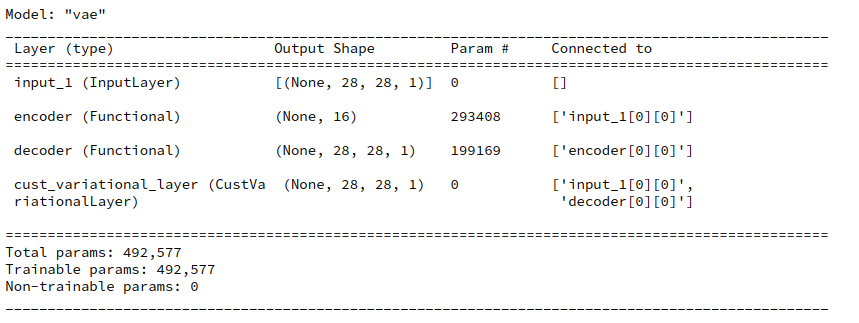
Now, we add a special layer based on the above class and use it in the definition of a VAE model. I follow the code in F. Cholet’s book; there the customized layer concludes the layer structure after the Encoder and the Decoder:
enc_output = encoder(encoder_input)
decoder_output = decoder(enc_output)

# add the custom layer to the model
fc = CustVariationalLayer()([encoder_input, decoder_output])

vae = Model(encoder_input, fc, name="vae")
vae.summary()
The output fits the expectations
Eventually we need to compile. F. Chollet in his book from 2017 defines the loss as “None” because it is covered already by the layer.
vae.compile(optimizer=Adam(), loss=None)
fit() fails … a typical error message
We are ready to train – at least I thought so … We start training with scaled x_train images coming e.g. from the MNIST dataset by the following statements :
n_epochs = 3;
batch_size = 128
vae.fit( x=x_train, y=None, shuffle=True,
         epochs = n_epochs, batch_size=batch_size)
Unfortunately we get the following typical
Error message:
TypeError: You are passing KerasTensor(type_spec=TensorSpec(shape=(), dtype=tf.float32, name=None), name='tf.math.reduce_sum_1/Sum:0', description="created by layer 'tf.math.reduce_sum_1'"), an intermediate Keras symbolic input/output, to a TF API that does not allow registering custom dispatchers, such as `tf.cond`, `tf.function`, gradient tapes, or `tf.map_fn`. Keras Functional model construction only supports TF API calls that *do* support dispatching, such as `tf.math.add` or `tf.reshape`. Other APIs cannot be called directly on symbolic Kerasinputs/outputs. You can work around this limitation by putting the operation in a custom Keras layer `call` and calling that layer on this symbolic input/output.
The error is due to “eager execution”!
The problem I experienced was related to a concise “eager mode execution” implemented in Tensorflow ≥ 2.3. If we deactivate “eager execution” by the following statement before we define any layers
from tensorflow.python.framework.ops import disable_eager_execution
disable_eager_execution()
then we get
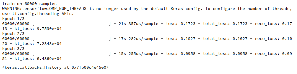
You can safely ignore the warning which is due to a superfluous environment variable.
And the other approaches for the KL loss?
Addendum 25.05.2022: This paragraph had to be changed as its original version contained wrong statements.
I had and have code examples for all the four variants of implementing the KL loss listed above. Both methods 1 and 2 do NOT work with standard TF 2.7 or 2.8 and active “eager execution” mode. Similar error messages as described for method 2 came up when I tried the original code of D. Foster, which you can download from his github repository. However, methods 3 and 4 do work – as long as you avoid any intermediate function to calculate the KL loss.
Important remark about F. Chollet’s present solution:
I should add that F. Chollet has, of course, meanwhile published a modern and working approach in the present online Keras documentation. I shall address his actual solution in a later post. His book is also the oldest of the four referenced.
Conclusion
In this post we have invested a lot of effort to realize a Keras model for a VAE – including the Kullback-Leibler loss. We have followed recipes of various books on Machine Learning. Unfortunately, we have to face a challenge:
Recipes of how to implement the KL loss for VAEs in books which are older than ca. 2 years may not work any longer with present versions of Tensorflow 2 and its “eager execution mode”.
In the next post of this series
Variational Autoencoder with Tensorflow – IV – simple rules to avoid problems with eager execution
we shall have a closer look at the problem. I will try to derive a central rule which will be helpful for the design various solutions that do work with TF 2.8.
Literature references
F. Chollet, Deep Learning mit Python und Keras, 2018, 1-te dt. Auflage, mitp Verlags GmbH & Co.KG, Frechen
D. Foster, “Generatives Deep Learning”, 2020, 1-te dt. Auflage, dpunkt Verlag, Heidelberg in Kooperation mit Media Inc.O’Reilly, ISBN 978-3-960009-128-8. See Kap. 3 and the VAE code published at
https://github.com/ davidADSP/ GDL_code/
A. Geron, “Hands-On Machine Learning with Scikit-Learn, keras & Tensorflow”, 2019, 2nd edition, O’Reilly, Sebastpol, Canada, ISBN 978-1-492-03264-9. See chapter 17.
R. Atienza, “Advanced Deep Learniing with Tensorflow 2 and Keras, 2020, 2nd edition, Packt Publishing, Birminham, UK, ISBN 978-1-83882-165-4. See chapter 8.
Ceterum censeo: The worst living fascist and war criminal today, who must be isolated, denazified and imprisoned, is the Putler.