I continue with my series on options of how to handle the KL loss in Variational Autoencoders [VAEs] in a Tensorflow 2 environment with eager execution:
Variational Autoencoder with Tensorflow – I – some basics
Variational Autoencoder with Tensorflow – II – an Autoencoder with binary-crossentropy loss
Variational Autoencoder with Tensorflow – III – problems with the KL loss and eager execution
Variational Autoencoder with Tensorflow – IV – simple rules to avoid problems with eager execution
Variational Autoencoder with Tensorflow – V – a customized Encoder layer for the KL loss
In the last post we delegated the KL loss calculation to a special customized layer of the Encoder. The layer directly followed two Dense layers which produced the tensors for
- the mean values mu
- and the logarithms of the variances log_var
of statistical standard distributions for z-points in the latent space. (Keep in mind that we have one mu and log_var for each sample. The KL loss function has a compactification impact on the z-point distribution as a whole and a normalization effect regarding the distribution around each z-point.)
The layer centered approach for the KL loss proved to be both elegant and fast in combination with Tensorflow 2. And it fits very well to the way we build ANNs with Keras.
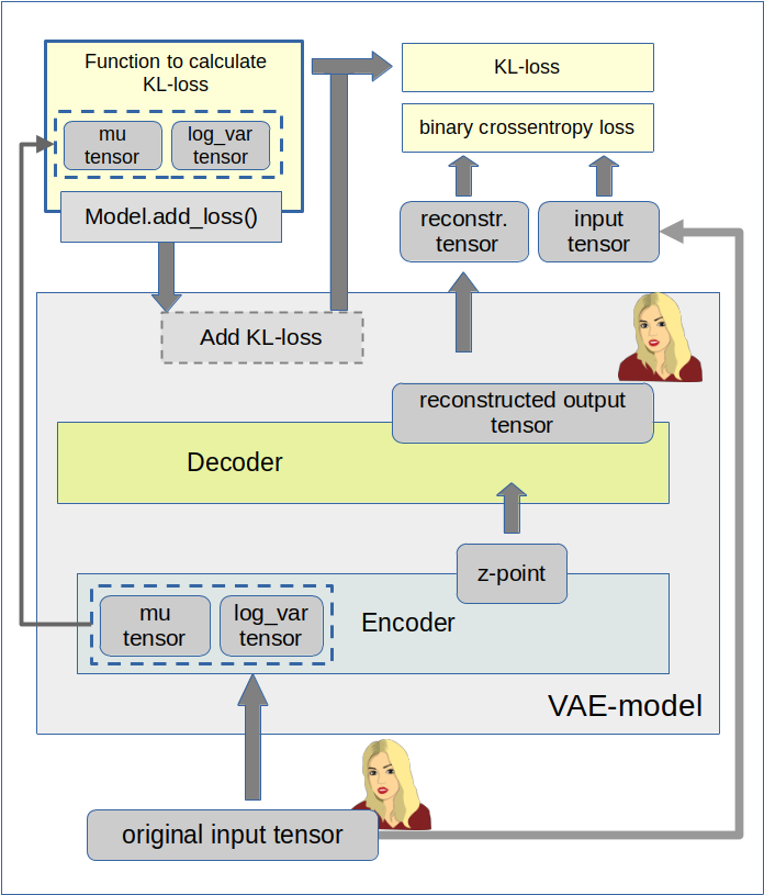
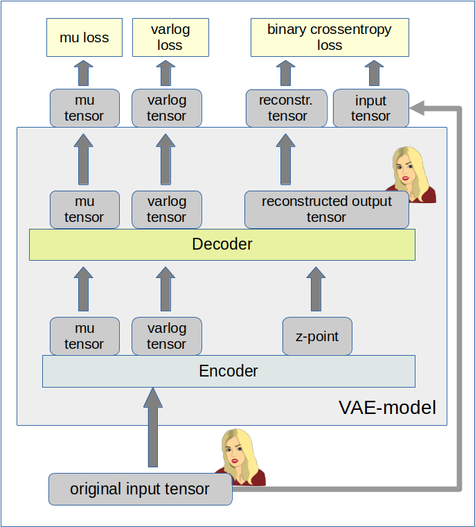
In the present post I focus on a different and more complicated strategy: We shall couple the Encoder and the Decoder by multi-output and multi-input interfaces to transfer mu and log_var tensors to the output side of our VAE model. And then we will calculate the KL loss by using a Keras standard mechanism for costs related to multiple output channels:
We can define a standardized customizable cost function per output channel (= per individual output tensor). Such a Keras cost function accepts two standard input variables: a predicted output tensor for the output channel and a related tensor with true values.
Such costs will automatically be added up to get a total loss and they will be subject to automatic error back propagation under eager execution conditions. However, to use this mechanism requires to transport KL related tensors to the Decoder’s output side and to split the KL loss into components.
The approach is a bit of an overkill to handle the KL loss. But it will also sheds a light on
- multi-in- and multi-output models
- multi-loss models
- and a transfer of tensors between to co-working neural nets.
Therefore the approach is interesting beyond VAE purposes.
Below I will first explain some more details of the present strategy. Afterward we need to find out how to handle standard customized Keras cost-functions for the KL loss contributions and the main loss. Furthermore we have to deal with reasonable output for the different loss terms during the training epochs. A performance comparison will show that the solution – though complicated – is a fast one.
The strategy in more details: A transfer variational KL tensors from the Encoder to the Decoder
First a general reminder: During training of a Keras model we have to guarantee a correct calculation of partial derivatives of losses with respect to trainable parameters (weights) according to the chain rule. The losses and related tensors themselves depend on matrix operations involving the layers’ weights and activation functions. So the chain rule has to be applied along all paths through the network. With eager execution all required operations and tensors must already be totally clear during a forward pass to the layers. We saw this already with the solution approach which we discussed in
Variational Autoencoder with Tensorflow 2.8 – IV – simple rules to avoid problems with eager execution
This means that relevant tensors must explicitly be available whenever derivatives shall be handled or pre-defined. This in turn means: When we want to calculate cost contributions after the definition of the full VAE model then we must transfer all required tensors down the line. Wth the functional Keras API we could use them by a direct Python reference to a layer. The alternative is to use them as explicit output of our VAE-model.
The strategy of this post is basically guided by a general Keras rule:
A personally customized cost function which can effortlessly be used in the compile()-statement for a Keras model in an eager execution environment should have a standard interface given by
cost_function( y_true, y_pred )
With exactly these two tensors as parameters – and nothing else!
See https://keras.io/api/losses/#creating-custom-losses. Such a function can be used for each of the multiple outputs of a Keras model.
One reason for this strict rule is that with eager execution the dependence of any function on input variables (tensors) must explicitly be defined via the function’s interface. For a standardized interface of a customizable model’s cost function the necessary steps can be generalized. The advantage of invoking cost functions with standardized interfaces for multiple output channels is, of course, the ease of use.
In the case of an Autoencoder the dominant predicted output is the (reconstructed) output tensor calculated from a z-point by the Decoder. By a comparison of this output tensor (e.g. a reconstructed image) with the original input tensor of the Encoder (e.g. an original image) a value for the binary crossentropy loss can be calculated. We extend this idea about output tensors of the VAE model now to the KL related tensors:
When you look at the KL loss definition in the previous posts with respect to mu and log_var tensors of the Encoder
kl_loss = -0.5e-4 * tf.reduce_mean(1 + log_var - tf.square(mu) - tf.exp(log_var))
you see that we can split it in log_var- and mu-dependent terms. If we could transfer the mu and log_var tensors from the Encoder part to the Decoder part of a VAE we could use these tensors as explicit output of the VAE-model and thus as input for the simple standardized Keras loss functions. Without having to take any further care of eager execution requirements …
So: Why not use
- a multiple-output model for the Encoder, which then provides z-points plus mu and log_var tensors,
- a multiple-input, multiple-output model for the Decoder, which then accepts the multiple output tensors of the Encoder as input and provides a reconstruction tensor plus the mu and log_var tensors as multiple outputs
- and simple customizable Keras cost-functions in the compile() statement for the VAE-model with each function handling one of the VAE’s (= Decoder’s) multiple outputs afterward?
Changes to the class MyVariationalAutoencoder
In the last post I have already described a class which handles all model-setup operations. We are keeping the general structure of the class – but we allow now for options in various methods to realize a different solution based on our present strategy. We shall use the input variable “solution_type” to the __init__() function for controlling the differences. The __init__() function itself can remain as it was defined in the last post.
Changes to the Encoder
We change the method to build the encoder of the class “MyVariationalAutoencoder” in the following way:
    # Method to build the Encoder
    # ~~~~~~~~~~~~~~~~~~~~~~~~~~~
    def _build_enc(self, solution_type = -1, fact=-1.0):

        # Checking whether "fact" and "solution_type" for the KL loss shall be overwritten
        if fact < 0:
            fact = self.fact
        if solution_type < 0:
            solution_type = self.solution_type
        else:
            self.solution_type = solution_type

        # Preparation: We later need a function to calculate the z-points in the latent space
        # The following function will be used by an eventual Lambda layer of the Encoder
        def z_point_sampling(args):
            '''
            A point in the latent space is calculated statistically
            around an optimized mu for each sample
            '''
            mu, log_var = args # Note: These are 1D tensors !
            epsilon = B.random_normal(shape=B.shape(mu), mean=0., stddev=1.)
            return mu + B.exp(log_var / 2) * epsilon


        # Input "layer"
        self._encoder_input = Input(shape=self.input_dim, name='encoder_input')

        # Initialization of a running variable x for individual layers
        x = self._encoder_input

        # Build the CNN-part with Conv2D layers
        # Note that stride>=2 reduces spatial resolution without the help of pooling layers
        for i in range(self.n_layers_encoder):
            conv_layer = Conv2D(
                filters = self.encoder_conv_filters[i]
                , kernel_size = self.encoder_conv_kernel_size[i]
                , strides = self.encoder_conv_strides[i]
                , padding = 'same'  # Important ! Controls the shape of the layer tensors.
                , name = 'encoder_conv_' + str(i)
                )
            x = conv_layer(x)

            # The "normalization" should be done ahead of the "activation"
            if self.use_batch_norm:
                x = BatchNormalization()(x)

            # Selection of activation function (out of 3)
            if self.act == 0:
                x = LeakyReLU()(x)
            elif self.act == 1:
                x = ReLU()(x)
            elif self.act == 2:
                # RMO: Just use the Activation layer to use SELU with predefined (!) parameters
                x = Activation('selu')(x)

            # Fulfill some SELU requirements
            if self.use_dropout:
                if self.act == 2:
                    x = AlphaDropout(rate = 0.25)(x)
                else:
                    x = Dropout(rate = 0.25)(x)

        # Last multi-dim tensor shape - is later needed by the decoder
        self._shape_before_flattening = B.int_shape(x)[1:]

        # Flattened layer before calculating VAE-output (z-points) via 2 special layers
        x = Flatten()(x)

        # "Variational" part - create 2 Dense layers for a statistical distribution of z-points
        self.mu      = Dense(self.z_dim, name='mu')(x)
        self.log_var = Dense(self.z_dim, name='log_var')(x)

        if solution_type == 0:
            # Customized layer for the calculation of the KL loss based on mu, var_log data
            # We use a customized layer according to a class definition
            self.mu, self.log_var = My_KL_Layer()([self.mu, self.log_var], fact=fact)

        # Layer to provide a z_point in the Latent Space for each sample of the batch
        self._encoder_output = Lambda(z_point_sampling, name='encoder_output')([self.mu, self.log_var])

        # The Encoder Model
        # ~~~~~~~~~~~~~~~~~~~
        # With KL -layer
        if solution_type == 0:
            self.encoder = Model(self._encoder_input, self._encoder_output)

         # With transfer solution => Multiple outputs
        if solution_type == 1:
            self.encoder = Model(inputs=self._encoder_input, outputs=[self._encoder_output, self.mu, self.log_var], name="encoder")
            # Other option
            #self.enc_inputs = {'mod_ip': self._encoder_input}
            #self.encoder = Model(inputs=self.enc_inputs, outputs=[self._encoder_output, self.mu, self.log_var], name="encoder")
For our present approach those parts are relevant which depend on the condition “solution_type == 1”.
Hint: Note that we could have used a dictionary to describe the input to the Encoder. In more complex models this may be reasonable to achieve formal consistency with the multiple outputs of the VAE-model which will often be described by a dictionary. In addition the losses and metrics of the VAE-model will also be handled by dictionaries. By the way: The outputs as well the respective cost and metric assignments of a Keras model must all be controlled by the same class of a Python enumerator.
The Encoder’s multi-output is described by a Python list of 3 tensors: The encoded z-point vectors (length: z_dim!), the mu- and the log_var 1D-tensors (length: z_dim!). (Note that the full shape of all tensors also depends on the batch-size during training where these tensors are of rank 2.) We can safely use a list here as we do not couple this output directly with VAE loss functions or metrics controlled by dictionaries. We use dictionaries only in the output definitions of the VAE model itself.
Changes to the Decoder
Now we must realize the transfer of the mu and log_var tensors to the Decoder. We have to change the Decoder into a multi-input model:
    # Method to build the Decoder
    # ~~~~~~~~~~~~~~~~~~~~~~~~~~~
    def _build_dec(self):

        # 1st Input layer - aligned to the shape of z-points in the latent space = output[0] of the Encoder
        self._decoder_inp_z = Input(shape=(self.z_dim,), name='decoder_input')

        # Additional Input layers for the KL tensors (mu, log_var) from the Encoder
        if self.solution_type == 1:
            self._dec_inp_mu       = Input(shape=(self.z_dim), name='mu_input')
            self._dec_inp_var_log  = Input(shape=(self.z_dim), name='logvar_input')

            # We give the layers later used as output a name
            # Each of the Activation layers below just corresponds to an identity passed through
            self._dec_mu            = Activation('linear',name='dc_mu')(self._dec_inp_mu)
            self._dec_var_log       = Activation('linear', name='dc_var')(self._dec_inp_var_log)

        # Nxt we use the tensor shape info from the Encoder
        x = Dense(np.prod(self._shape_before_flattening))(self._decoder_inp_z)
        x = Reshape(self._shape_before_flattening)(x)

        # The inverse CNN
        for i in range(self.n_layers_decoder):
            conv_t_layer = Conv2DTranspose(
                filters = self.decoder_conv_t_filters[i]
                , kernel_size = self.decoder_conv_t_kernel_size[i]
                , strides = self.decoder_conv_t_strides[i]
                , padding = 'same' # Important ! Controls the shape of tensors during reconstruction
                                   # we want an image with the same resolution as the original input
                , name = 'decoder_conv_t_' + str(i)
                )
            x = conv_t_layer(x)

            # Normalization and Activation
            if i < self.n_layers_decoder - 1:
                # Also in the decoder: normalization before activation
                if self.use_batch_norm:
                    x = BatchNormalization()(x)

                # Choice of activation function
                if self.act == 0:
                    x = LeakyReLU()(x)
                elif self.act == 1:
                    x = ReLU()(x)
                elif self.act == 2:
                    #x = self.selu_scale * ELU(alpha=self.selu_alpha)(x)
                    x = Activation('selu')(x)

                # Adaptions to SELU requirements
                if self.use_dropout:
                    if self.act == 2:
                        x = AlphaDropout(rate = 0.25)(x)
                    else:
                        x = Dropout(rate = 0.25)(x)

            # Last layer => Sigmoid output
            # => This requires scaled input => Division of pixel values by 255
            else:
                x = Activation('sigmoid', name='dc_reco')(x)

        # Output tensor => a scaled image
        self._decoder_output = x

        # The Decoder model

        # solution_type == 0: Just the decoded input
        if self.solution_type == 0:
            self.decoder = Model(self._decoder_inp_z, self._decoder_output)

        # solution_type == 1: The decoded tensor plus
        #                     plus the transferred tensors mu and log_var a for the variational distributions
        if self.solution_type == 1:
            self.decoder = Model([self._decoder_inp_z, self._dec_inp_mu, self._dec_inp_var_log],
                                 [self._decoder_output, self._dec_mu, self._dec_var_log], name="decoder")
You see that the Decoder has evolved into a “multi-input, multi-output model” for “solution_type==1”.
Construction of the VAE model
Next we define the full VAE model. We want to organize its multiple outputs and align them with distinct loss functions and maybe also some metrics information. I find it clearer to do this via dictionaries, which refer to layer names in a concise way.
    # Function to build the full VAE
    # ~~~~~~~~~~~~~~~~~~~~~~~~~~~~~~~~~~~~~~~~~~~~~
    def _build_VAE(self):

        solution_type = self.solution_type

        if solution_type == 0:
            model_input  = self._encoder_input
            model_output = self.decoder(self._encoder_output)
            self.model = Model(model_input, model_output, name="vae")

        if solution_type == 1:
            enc_out      = self.encoder(self._encoder_input)
            dc_reco, dc_mu, dc_var = self.decoder(enc_out)

            # We organize the output and later association of cost functions and metrics via a dictionary
            mod_outputs = {'vae_out_main': dc_reco, 'vae_out_mu': dc_mu, 'vae_out_var': dc_var}
            self.model = Model(inputs=self._encoder_input, outputs=mod_outputs, name="vae")

            # Another option if we had defined a dictionary for the encoder input
            #self.model = Model(inputs=self.enc_inputs, outputs=mod_outputs, name="vae")
Compilation and Costs
The next logical step is to define our cost contributions. I am going to do this as with the help of two sub-functions of a method leading to the compilation of the VAE-model.
    # Function to compile the full VAE
    # ~~~~~~~~~~~~~~~~~~~~~~~~~~~~~~~~~~~~~~~~~~~~~
    def compile_myVAE(self, learning_rate):
        # Optimizer
        optimizer = Adam(learning_rate=learning_rate)
        # save the learning rate for possible intermediate output to files
        self.learning_rate = learning_rate

        # Parameter "fact" will be used by the cost functions defined below to scale the KL loss relative to the BCE loss
        fact = self.fact

        #mu-dependent cost contributions to the KL loss
        @tf.function
        def mu_loss(y_true, y_pred):
            loss_mux = fact * tf.reduce_mean(tf.square(y_pred))
            return loss_mux

        #log_var dependent cost contributions to the KL loss
        @tf.function
        def logvar_loss(y_true, y_pred):
            loss_varx = -fact * tf.reduce_mean(1 + y_pred - tf.exp(y_pred))
            return loss_varx

        # Model compilation
        # ~~~~~~~~~~~~~~~~~~~~
        if self.solution_type == 0:
            self.model.compile(optimizer=optimizer, loss="binary_crossentropy",
                               metrics=[tf.keras.metrics.BinaryCrossentropy(name='bce')])

        if self.solution_type == 1:
            self.model.compile(optimizer=optimizer
                               , loss={'vae_out_main':'binary_crossentropy', 'vae_out_mu':mu_loss, 'vae_out_var':logvar_loss}
                              #, metrics={'vae_out_main':tf.keras.metrics.BinaryCrossentropy(name='bce'), 'vae_out_mu':mu_loss, 'vae_out_var': logvar_loss }
                               )
The first interesting thing is that the statements inside the two cost functions ignore “y_true” completely. Unfortunately, a small test shows that we nevertheless must provide some reasonable dummy tensors here. “None” is NOT working in this case.
The dictionary organizes the different costs and their relation to the three output channels of our VAE-model. I have included the metrics as a comment for the moment. It would only produce double output and consume a bit of performance.
A method for training and fit()
To enable training we use the following function:
    def train_myVAE(self, x_train, batch_size, epochs, initial_epoch = 0, t_mu=None, t_logvar=None ):

        if self.solution_type == 0:
            self.model.fit(
                x_train
                , x_train
                , batch_size = batch_size
                , shuffle = True
                , epochs = epochs
                , initial_epoch = initial_epoch
            )
        if self.solution_type == 1:
            self.model.fit(
                x_train
                # , [x_train, t_mu, t_logvar] # we provide some dummy tensors here
                , {'vae_out_main': x_train, 'vae_out_mu': t_mu, 'vae_out_var':t_logvar}
                , batch_size = batch_size
                , shuffle = True
                , epochs = epochs
                , initial_epoch = initial_epoch
            )
You may wonder what the “t_mu” and “t_log_var” stand for. These are the dummy tensors which have to provide to the cost functions. The fit() function gets “x_train” as the model’s input. The tensors “y_pred”, for which we optimize, are handed over to the three loss functions by
{ 'vae_out_main': x_train, 'vae_out_mu': t_mu, 'vae_out_var':t_logvar}
Again, I have organized the correct association to each output and loss contribution via a dictionary.
Testing
We can use the same Jupyter notebook with almost the same cells as in my last post V. An adaption is only required for the cells starting the training.
I build a “vae” object (which can later be used for the MNIST dataset) by
Cell 6
from my_AE_code.models.MyVAE_2 import MyVariationalAutoencoder

z_dim = 2
vae = MyVariationalAutoencoder(
    input_dim = (28,28,1)
    , encoder_conv_filters = [32,64,128]
    , encoder_conv_kernel_size = [3,3,3]
    , encoder_conv_strides = [1,2,2]
    , decoder_conv_t_filters = [64,32,1]
    , decoder_conv_t_kernel_size = [3,3,3]
    , decoder_conv_t_strides = [2,2,1]
    , z_dim = z_dim
    , solution_type = 1  # now we must provide the solution type - here the solution with KL tensor Transfer
    , act   = 0
    , fact  = 1.e-3
)
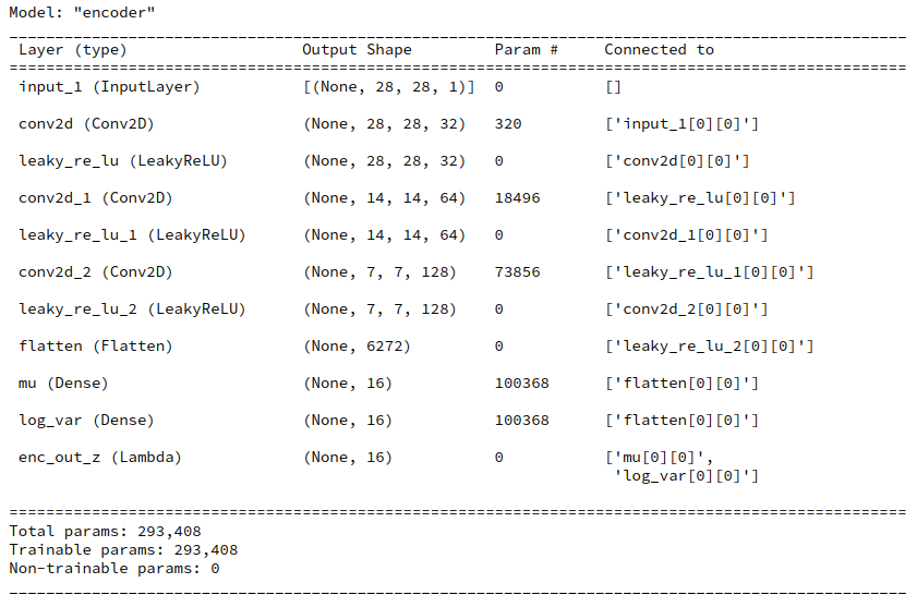
Afterwards I use the Jupyter cells presented in my last post to build the Encoder, the Decoder and then the full VAE-model. For z_dim = 2 the summary outputs for the models now look like:
Encoder
Model: "encoder"
__________________________________________________________________________________________________
 Layer (type)                   Output Shape         Param #     Connected to
==================================================================================================
 encoder_input (InputLayer)     [(None, 28, 28, 1)]  0           []

 encoder_conv_0 (Conv2D)        (None, 28, 28, 32)   320         ['encoder_input[0][0]']

 leaky_re_lu_15 (LeakyReLU)     (None, 28, 28, 32)   0           ['encoder_conv_0[0][0]']

 encoder_conv_1 (Conv2D)        (None, 14, 14, 64)   18496       ['leaky_re_lu_15[0][0]']

 leaky_re_lu_16 (LeakyReLU)     (None, 14, 14, 64)   0           ['encoder_conv_1[0][0]']

 encoder_conv_2 (Conv2D)        (None, 7, 7, 128)    73856       ['leaky_re_lu_16[0][0]']

 leaky_re_lu_17 (LeakyReLU)     (None, 7, 7, 128)    0           ['encoder_conv_2[0][0]']

 flatten_3 (Flatten)            (None, 6272)         0           ['leaky_re_lu_17[0][0]']

 mu (Dense)                     (None, 2)            12546       ['flatten_3[0][0]']

 log_var (Dense)                (None, 2)            12546       ['flatten_3[0][0]']

 encoder_output (Lambda)        (None, 2)            0           ['mu[0][0]',
                                                                  'log_var[0][0]']

==================================================================================================
Total params: 117,764
Trainable params: 117,764
Non-trainable params: 0
__________________________________________________________________________________________________
Decoder
Model: "decoder"
__________________________________________________________________________________________________
 Layer (type)                   Output Shape         Param #     Connected to
==================================================================================================
 decoder_input (InputLayer)     [(None, 2)]          0           []

 dense_4 (Dense)                (None, 6272)         18816       ['decoder_input[0][0]']

 reshape_4 (Reshape)            (None, 7, 7, 128)    0           ['dense_4[0][0]']

 decoder_conv_t_0 (Conv2DTransp  (None, 14, 14, 64)  73792       ['reshape_4[0][0]']
 ose)

 leaky_re_lu_23 (LeakyReLU)     (None, 14, 14, 64)   0           ['decoder_conv_t_0[0][0]']

 decoder_conv_t_1 (Conv2DTransp  (None, 28, 28, 32)  18464       ['leaky_re_lu_23[0][0]']
 ose)

 leaky_re_lu_24 (LeakyReLU)     (None, 28, 28, 32)   0           ['decoder_conv_t_1[0][0]']

 decoder_conv_t_2 (Conv2DTransp  (None, 28, 28, 1)   289         ['leaky_re_lu_24[0][0]']
 ose)

 mu_input (InputLayer)          [(None, 2)]          0           []

 logvar_input (InputLayer)      [(None, 2)]          0           []

 dc_reco (Activation)           (None, 28, 28, 1)    0           ['decoder_conv_t_2[0][0]']

 dc_mu (Activation)             (None, 2)            0           ['mu_input[0][0]']

 dc_var (Activation)            (None, 2)            0           ['logvar_input[0][0]']

==================================================================================================
Total params: 111,361
Trainable params: 111,361
Non-trainable params: 0
__________________________________________________________________________________________________
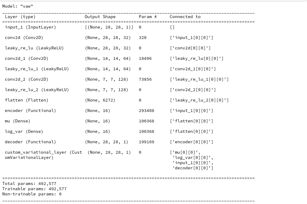
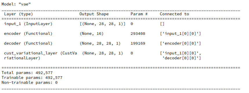
VAE-model
Model: "vae"
__________________________________________________________________________________________________
 Layer (type)                   Output Shape         Param #     Connected to                      height: 200px; overflow:auto;
==================================================================================================
 encoder_input (InputLayer)     [(None, 28, 28, 1)]  0           []

 encoder (Functional)           [(None, 2),          117764      ['encoder_input[0][0]']
                                 (None, 2),
                                 (None, 2)]

 model_3 (Functional)           [(None, 28, 28, 1),  111361      ['encoder[0][0]',
                                 (None, 2),                       'encoder[0][1]',
                                 (None, 2)]                       'encoder[0][2]']

==================================================================================================
Total params: 229,125
Trainable params: 229,125
Non-trainable params: 0
__________________________________________________________________________________________________
We can use our modified class in a Jupyter notebook in the same way as I have discussed in the last . Of course you have to adapt the cells slightly; the parameter solution_type must be set to 1:
Training can be started with some dummy tensors for “y_true” handed over to our two special cost functions for the KL loss as:
Cell 11
BATCH_SIZE = 128
EPOCHS = 6
PRINT_EVERY_N_BATCHES = 100
INITIAL_EPOCH = 0

# Dummy tensors
t_mu     = tf.convert_to_tensor(np.zeros((60000, z_dim), dtype='float32'))
t_logvar = tf.convert_to_tensor(np.ones((60000, z_dim), dtype='float32'))

vae.train_myVAE(
    x_train[0:60000]
    , batch_size = BATCH_SIZE
    , epochs = EPOCHS
    , initial_epoch = INITIAL_EPOCH
   , t_mu = t_mu
   , t_logvar = t_logvar
)
Note that I have provided dummy tensors with a shape fitting the length of x_train (60,000) and the other dimension as z_dim! This, of course, costs some memory ….
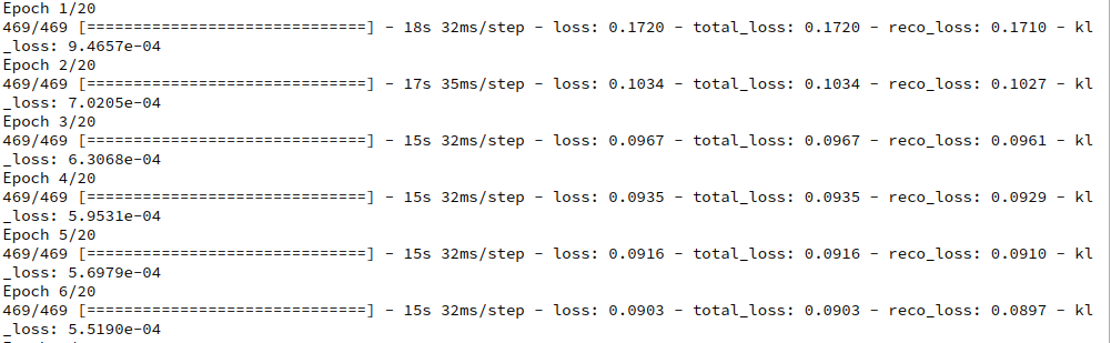
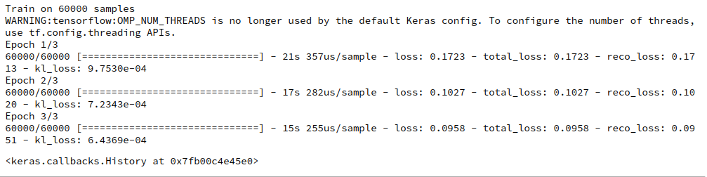
As output we get:
Epoch 1/6
469/469 [==============================] - 14s 23ms/step - loss: 0.2625 - decoder_loss: 0.2575 - decoder_1_loss: 0.0017 - decoder_2_loss: 0.0032
Epoch 2/6
469/469 [==============================] - 12s 25ms/step - loss: 0.2205 - decoder_loss: 0.2159 - decoder_1_loss: 0.0013 - decoder_2_loss: 0.0032
Epoch 3/6
469/469 [==============================] - 11s 22ms/step - loss: 0.2137 - decoder_loss: 0.2089 - decoder_1_loss: 0.0014 - decoder_2_loss: 0.0034
Epoch 4/6
469/469 [==============================] - 11s 23ms/step - loss: 0.2100 - decoder_loss: 0.2050 - decoder_1_loss: 0.0013 - decoder_2_loss: 0.0037
Epoch 5/6
469/469 [==============================] - 10s 22ms/step - loss: 0.2072 - decoder_loss: 0.2021 - decoder_1_loss: 0.0013 - decoder_2_loss: 0.0039
Epoch 6/6
469/469 [==============================] - 10s 22ms/step - loss: 0.2049 - decoder_loss: 0.1996 - decoder_1_loss: 0.0013 - decoder_2_loss: 0.0041
Heureka, our complicated setup works!
And note: It is fast! Just compare the later epoch times to the ones we got in the last post. 10 ms compared to 11 ms per epoch!
Getting clearer names for the various losses?
One thing which is not convincing is the fact that Keras provides all losses with some standard (non-speaking) names. To make things clearer you could
- either define some loss related metrics for which you define understandable names
- or invoke a customized Callback and maybe stop the standard output.
With the metrics you will get double output – the losses with standard names and once again with you own names. And it will cost a bit of performance.
The standard output of Keras can be stopped by a parameter “verbose=0” of the train()-function. However, this will stop the progress bar, too.
I did not find any simple solution so far for this problem of customizing the output. If you do not need a progress bar then just set “verbose = 0” and use your own Callback to control the output. Note that you should first look at the available keys for logged output in a test run first. Below I give you the code for your own experiments:
    def train_myVAE(self, x_train, batch_size, epochs, initial_epoch = 0, t_mu=None, t_logvar=None ):

        class MyPrinterCallback(tf.keras.callbacks.Callback):

            # def on_train_batch_begin(self, batch, logs=None):
            #     # Do something on begin of training batch

            def on_epoch_end(self, epoch, logs=None):

                # Get overview over available keys
                #keys = list(logs.keys())
                #print("End epoch {} of training; got log keys: {}".format(epoch, keys))

                print("\nEPOCH: {}, Total Loss: {:8.6f}, // reco loss: {:8.6f}, mu Loss: {:8.6f}, logvar loss: {:8.6f}".format(epoch,
                                                logs['loss'], logs['decoder_loss'], logs['decoder_1_loss'], logs['decoder_2_loss']
                                            ))
                print()

            def on_epoch_begin(self, epoch, logs=None):
                print('-'*50)
                print('STARTING EPOCH: {}'.format(epoch))

        if self.solution_type == 0:
            self.model.fit(
                x_train
                , x_train
                , batch_size = batch_size
                , shuffle = True
                , epochs = epochs
                , initial_epoch = initial_epoch
            )

        if self.solution_type == 1:
            self.model.fit(
                x_train
                #Exp.:
                , {'vae_out_main': x_train, 'vae_out_mu': t_mu, 'vae_out_var':t_logvar}
                , batch_size = batch_size
                , shuffle = True
                , epochs = epochs
                , initial_epoch = initial_epoch
                #, verbose=0
                , callbacks=[MyPrinterCallback()]
            )
Output example:
EPOCH: 2, Total Loss: 0.203891, // reco loss: 0.198510, mu Loss: 0.001242, logvar loss: 0.004139

469/469 [==============================] - 11s 23ms/step - loss: 0.2039 - decoder_loss: 0.1985 - decoder_1_loss: 0.0012 - decoder_2_loss: 0.0041
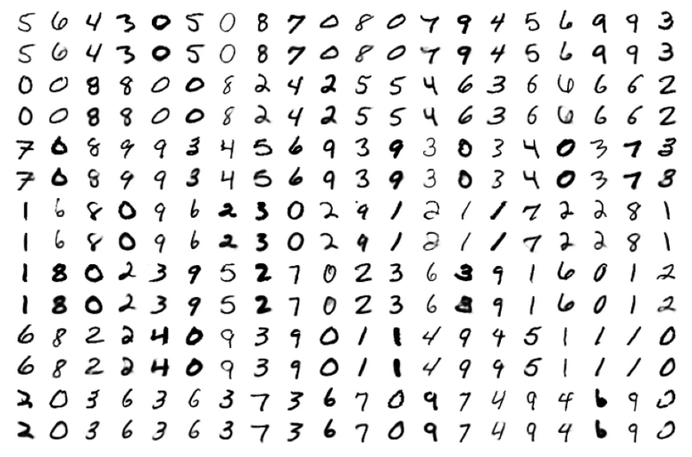
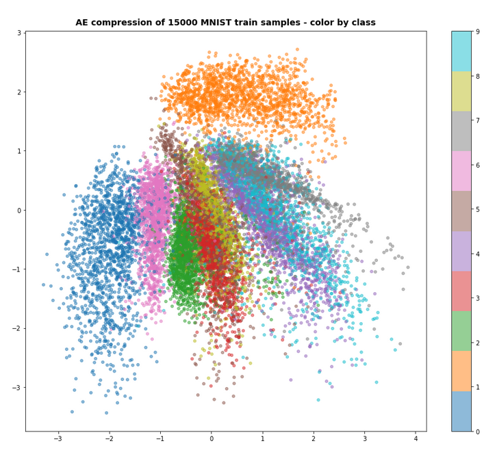
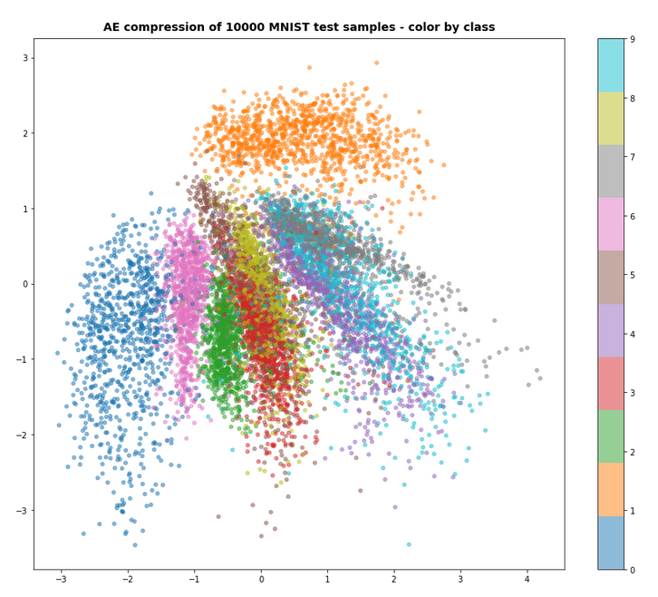
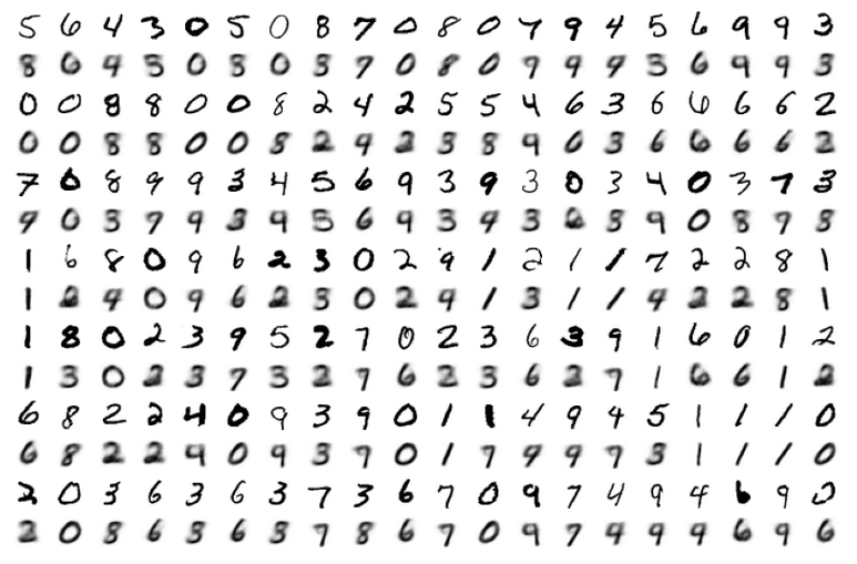
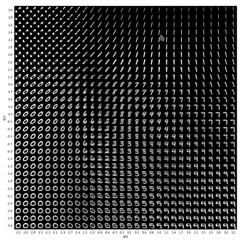
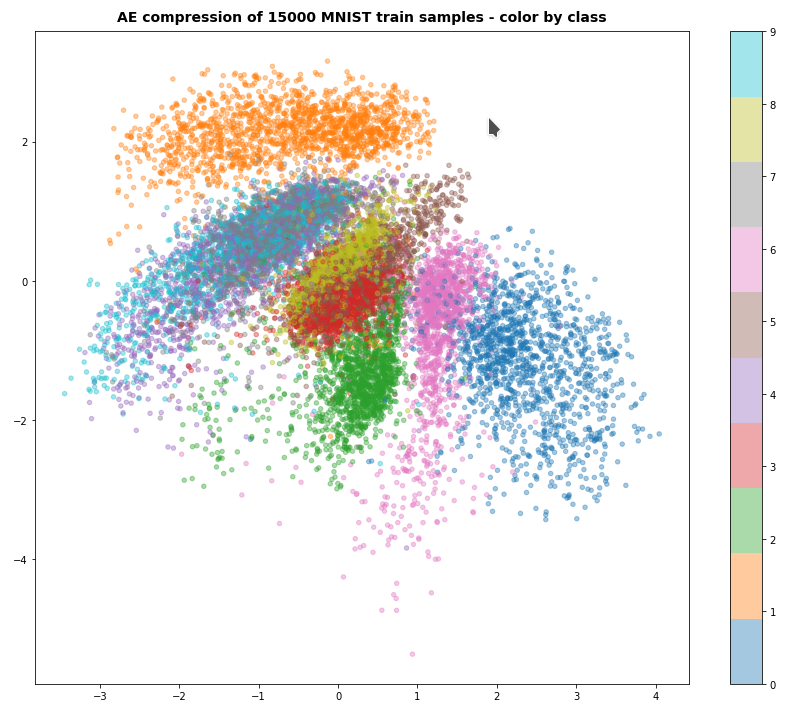
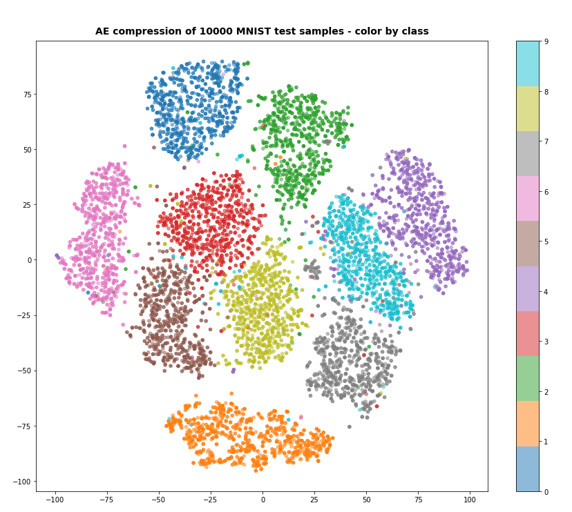
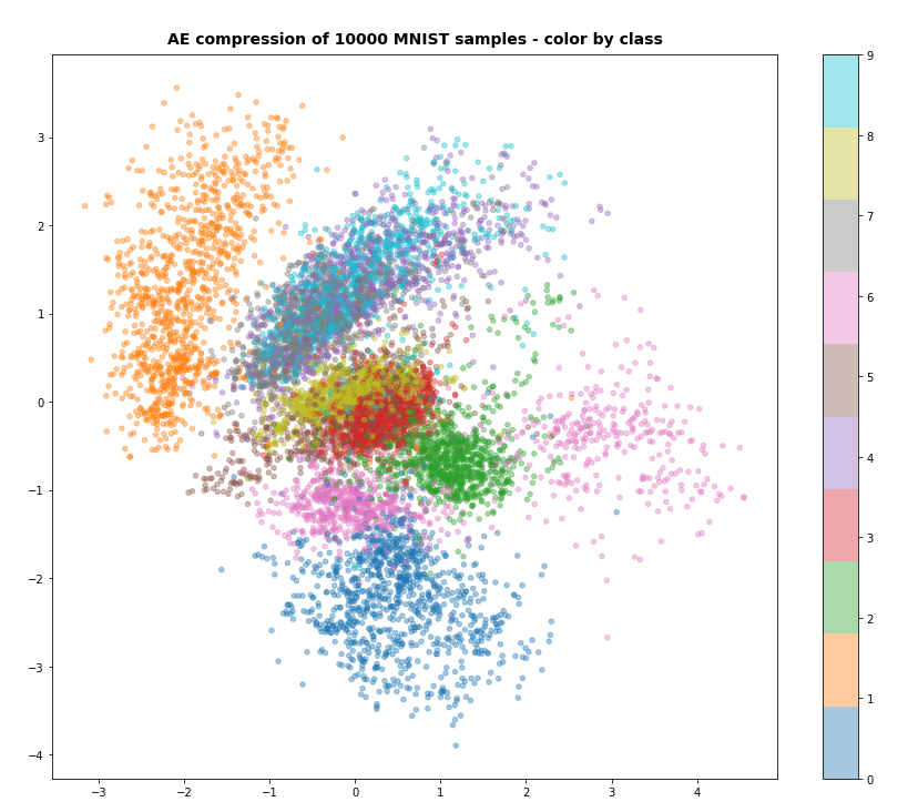
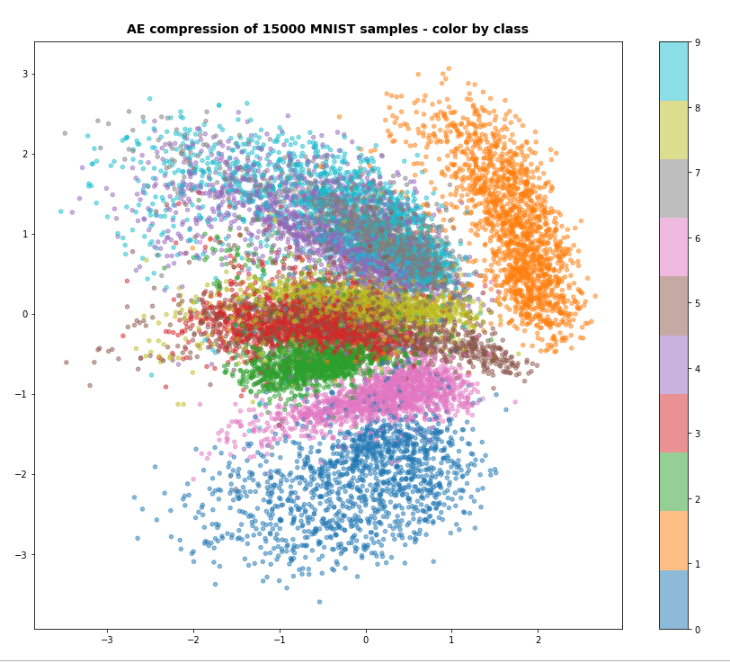
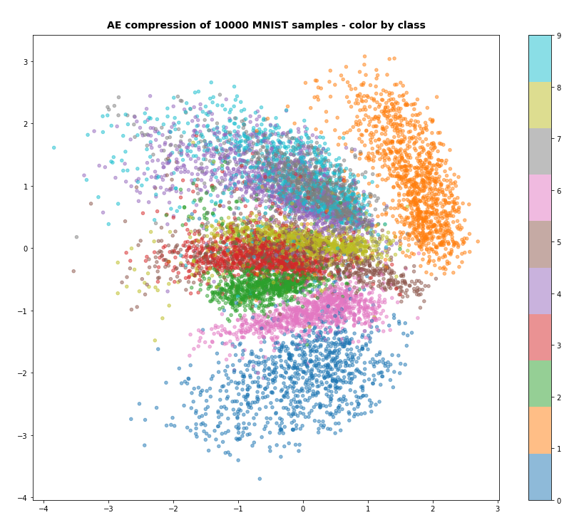
Output in the latent space
Just to show that the VAE is doing what is expected some out put from the latent space:
Conclusion
In this post we have used a standard option of Keras to define (eager execution compatible) loss functions. We transferred the KL loss related tensors “mu” and “logvar” to the Decoder and used them as different output tensors of our VAE-model. We needed to provide some dummy “y_true” tensors to the cost functions. The approach is a bit complicated, but it is working under eager execution conditions and it does not reduce performance.
It also provided us with some insights into coupled “multi-input/multi-output models” and cost handling for each of the outputs.
Still, this interesting approach appears as an overkill for handling the KL loss. In the next post
Variational Autoencoder with Tensorflow – VII – KL loss via model.add_loss()
I shall turn to a seemingly much lighter approach which will use the model.add_loss() functionality of Keras.
Ceterum censeo: The worst living fascist and war criminal today, who must be isolated, denazified and imprisoned, is the Putler.