In unserer Firma fallen z.Z. mehrere technische Schritte an, die wir parallel abwickeln müssen:
So stellen wir einerseits zwei Opensuse-Leap-Server für einen Kunden auf Debian-8-basierte vServer beim Hoster Strato um. Zeitgleich ersetzen wir das von uns unter Eclipse genutzte Versionsverwaltungssystem SVN durch Git und binden u.a. auch dabei einen der gehosteten vServer ein.
Damit wir und unser Kunde auf dem vServer
- das dortige Git-Server-Repository besser kontrollieren und verfolgen können,
- gelegentlich Branches anlegen und Merge-Aktionen durchführen können,
sollen auf dem vServer auch graphische GIT-Frontends zum Einsatz kommen. Z.B. “cola-git”, “qgit”, “giggle”. Ziel ist u.a. die Ansicht solcher Graphen wie in der nachfolgenden Abbildung:

Obwohl die Anwendung am Server läuft, wollen wir den Output natürlich auf dem Desktop unserer Arbeitsplatz-PCs oder denen des Kunden ansehen können.
So stellte sich uns also die Frage, wie man am schnellsten zu einem performanten graphischen Remote-Desktop für ein gehostetes “headless” System, also für ein System ohne echte eigene Grafik-Ressourcen, kommt. In unserem Fall zeigte sich, dass X2GO die richtige Wahl war und ist.
Nomenklatur – Remote Hosts, X-Server, X-Clients
Wir verwenden im weiteren Text die nachfolgende Nomenklatur, um Missverständnisse zu vermeiden. Bekanntermaßen ist ja beim X11-Protokoll die laufende Grafik-Anwendung ein “X-Client”. Das Umsetzungsprogramm, das aus den Grafik-Befehlen des Clients schließlich Fenster und grafische Inhalte auf den Bildschirm eines Linux-Desktops oder oder die Grafikstation eines Thin Client zaubert, ist hingegen der “X-Server”.
Die zuständigen Protokolle für den Datenaustausch zwischen X-Client und X-Server funktionieren auch über Netzwerke hinweg:
- Als “Remote-Host” bezeichne ich den vServer bei Strato. Dort laufen dann Linux-Anwendungen, die grafischen Output im Rahmen ihres Benutzerinterfaces anbieten (in unserem Beispiel GIT-Anwendungen mit GUI).
- Das Linux-System, von dem aus wir auf den vServer zugreifen, nenne ich “Arbeitsplatz-PC” oder kurz “PC”. Auf ihm läuft unter Linux selbstverständlich auch ein lokaler X-Server. Dieser dient wiederum einem Linux-Desktop – in meinem Fall KDE 5 – als technische Basis für die Integration grafischer Benutzerschnittstellen zu lokalen und entfernten Anwendungen.
- Die graphischen Programme wie “qgit”, die auf dem vServer (=Remote-Host) laufen und ihren Output wie grafische Anweisungen einem lokalen oder über das Internet auch einem entfernten X-Server zuweisen, nennen wir “Remote X-Clients”.
Bzgl. möglicher Lösungen für Remote-Desktop-Darstellungen auf einem Arbeitsplatz-PC ist es nicht von vornherein klar, wo und in welcher Form ein X-Server zum Einsatz kommt. Natürlich läuft auf einem normalen Linux-PC ein X-Server für eine grafische Oberfläche; das schließt aber nicht aus, dass auch auf dem Remote-System ein X-Server aktiv ist.
Ein Remote-X-Client-Programm könnte also einerseits mit einem (headless) X-Server auf dem Remote-Host zusammenarbeiten. Er könnte andererseits aber auch direkt mit dem X-Server am Arbeitsplatz-PC über das Internet interagieren (z.B. über ssh -X oder die explizite Vorgabe eines entfernten X-Servers samt Screen über die Umgebungsvariable “DISPLAY”).
Funktionsweise von VNC vs. X2Go
Der Vollständigkeit halber werfen wir deshalb auch einen kurzen Blick auf Unterschiede in der typischen Funktionsweise von VNC und X2Go. Man beachte, dass in beiden Fällen “Server”-Komponenten auf dem Remote-Host und “Client”-Komponenten auf dem Arbeitsplatz-PC zum Einsatz kommen; das ist gerade umgekehrt wie bei den X11-Komponenten:
- VNC: Auf dem Remote-Host kann theoretisch ein headless X-Server laufen, für dessen Implementierung ggf. die zu installierende Remote-Desktop-Umgebung (wie etwa ein VNC-Server-Modul) sorgen muss. Dessen Bilddaten-Output könnten dann über ein VNC-Programm abgegriffen und über das Internet an einen Arbeitsplatz-PC bei uns übertragen werden. Dort greift dann ein VNC-Client-Programm die Daten auf und blendet sie als lokaler X-Client über ein passendes Fenster in den grafischen Linux-Desktops des PCs ein.
- X2Go: Unter X2Go läuft auf dem Remote-Host der sog. “X2Go-Server”. Der nutzt essentielle Teile des X11-Protokolls um Daten und Grafikanweisungen an den X-Server eines Arbeitsplatz-PCs zu übertragen. Dort koppelt allerdings ein zwischengeschalteter “X2Go-Client” an den X11-Server des Arbeitsplatz-PCs an. (Unter Windows Clients ist ein geeigneter X11-Server bereitzustellen!). Im Unterschied zu ” ssh -X” oder einem direkten Remote Zugriff auf einen X11-Server werden von den zwischengeschalteten X2Go-Komponenten zusätzlich Kompressionsalgorithmen und Caches exzessiv genutzt und der Statusabgleich zwischen X11-Server und X11-Client auf das notwendige Minimum reduziert.
In beiden Fällen müssen die VNC- oder X2Go-Client-Komponenten natürlich die Keyboard- und Mausinteraktionen mit den relevanten Fenstern am Arbeitsplatz-PC abfangen und an die X-Clients auf dem Remote-Host übertragen.
Ich gehe nachfolgend von klassischen X-Servern (und nicht Wayland) aus. Wayland ist meines Wissens nicht mit X2Go kompatibel.
SSH -X als Alternative ?
Natürlich habe ich auf unserem Strato-vServer erstmal eine direkte grafische Datenübertragung zwischen den X-Clients der vServer und meinem Arbeitsplatz-PC mittels “ssh -X” ausprobiert. Dabei wird der Grafik-Output der X-Remote-Clients (über das zwischengeschaltete Internet) direkt vom X-Server am Arbeitsplatz-PC behandelt. Aber Qgit, Giggle und Co. sind doch schon recht komplexe Anwendungen, die mit einem X-Server relativ häufig relativ viele Informationen austauschen müssen.
Ich war mit der Performance überhaupt nicht zufrieden. Das Arbeiten an sich erwies sich zwar nicht als unmöglich; aber bei verschiedenen Schritten treten doch spürbare Wartezeiten auf – u.a. beim Aufbau von Verzeichnis- und Strukturbäumen. Die Durchführung von Änderungen war dann nicht wirklich bequem, sprich nicht flüssig möglich. Mein Eindruck war: Es wird eine deutlich bessere Kompression und Pufferung der Daten benötigt.
Probleme mit VNC – und Einschränkungen bzgl. der Desktop-Umgebung
Ich dachte als Nächstes natürlich an klassische VNC-Anwendungen (https://de.wikipedia.org/ wiki/ Virtual_Network_Computing), mit deren Hilfe man einen echten Remote-Desktop realisiert.
In LANs hatte ich früher schon mal TurboVNC eingesetzt. Ich hatte das damals als recht performant empfunden. Sogar der Einsatz von VirtualGL für Remote-Hosts, die mit einer 3D-Grafik-Karte ausgestattet waren, war möglich. Nun braucht man für einen Strato vServer und GIT-Frontends natürlich kein VirtualGL. Aber TurboVNC war ja auch sonst ganz OK – zumindest unter älteren Opensuse-Systemen.
Dennoch habe ich den Einsatz von TurboVNC auf einem Strato-vServer mit Debian nach ein paar Experimenten abgebrochen. Unter Debian 8 gab es (fast erwartungsgemäß) Probleme mit Gnome 3 (trotz vorhandener Mesa-Bibliotheken). Gnome 3 ist (wie KDE 5 auch) von Haus aus für VNC problematisch, da 3D-Fähigkeiten der Umgebung vorausgesetzt werden. Bei mir klappte der Start des Desktops trotz vorhandener Mesa-Bibliotheken und des lokalen VMware-Grafiktreibers des Virtuozzo-Containers für den Strato-vServer nicht.
Auch eine kurze Recherche im Internet zeigte: Der Einsatz von Gnome erfordert unter klassischen VNC-Servern (und auch unter TurboVNC) einfach viel zu viele Klimmzüge. Wie funktionabel und performant dagegen der in Gnome integrierte VNC-Server “vino” ist, habe ich in meinem Frust dann nicht mehr ausprobiert.
KDE 4 unter Debian 8 ging zwar unter TurboVNC; ich bekam aber keine Veränderung der Auflösung jenseits 1024x768px am TurboVNC-Client auf dem Arbeitsplatz-System hin. Der Zeitaufwand für das Rumprobieren wurde mir dann irgendwann zu groß. Das hatte zwei Konsequenzen:
- Als erstes reduzierte ich meine Anforderungen an eine Desktop-Umgebung kurzentschlossen auf LXDE und KDE4. Mit letzterem kennt sich auch unser Kunde in hinreichendem Maße aus.
- Als zweites konzentrierte ich mich auf die von Debian im Standardumfang mitgelieferten VNC-Pakete: “tightvnc” und “vnc4server”.
Ein Kurztest der beiden VNC-Varianten überzeugte mich aber hinsichtlich der Performance mit KDE 4 nicht; besonders nicht der vnc4server. Mit LXDE konnte ich dagegen ganz gut arbeiten.
KDE 4 ist halt ein Desktop-Schwergewicht, das den X11-Server je nach Desktop-Gestaltung laufend belastet. Dabei ist zu bedenken, dass die meisten VNC-Systeme auf dem Remote-Linux-System einen laufenden (headless) X11-Server brauchen, dessen Bilddaten dann abgegriffen und an einen VNC-Client auf einem lokalen PC übertragen werden. Das ist vom logischen Prozess-Ablauf her gesehen ein Umweg, weil neben dem X11-Server noch eine Zwischenschicht auf dem Remote-System ausgeführt werden muss. Die Bilddaten auf dem lokalen PC müssen zudem wieder in einem Fenster auf dem lokalen X11-Server dargestellt werden.
X2Go als Alternative ?
Wenn es denn hinreichend schnell funktionieren würde, würde man deshalb als Linuxer eigentlich immer gerne direkt Remote-X11 über SSH einsetzen. Auf dem Remote-System – hier also dem vServer – liefen dann Anwendungen, die als X-Window-Client-Programme ihre Daten und graphischen Steuerbefehle (über einen SSH-Tunnel) direkt an den aktuell laufenden X11-Server auf meinem Arbeitsplatz-PC übertragen. In unserem LAN klappt das auch wunderbar – sogar mit der Übertragung von 3D-Grafik-Daten. Da reicht die Bandbreite schon in einem Gigabit-Netz zur schnellen Datenübertragung völlig aus. Das gilt aber leider nicht unbedingt für Remote-Systeme im Internet zu denen die Bandbreite in beide Richtungen begrenzt ist. (Zumindest bei mir).
Dann fiel mir ein: Eine hinsichtlich Kompression, Caching und X11-Server/Client-Abgleich optimierte Variante des X11-Protokolls über ein Netzwerkverbindungen lieferte doch das NX3-Nomachine-Protokoll; es bildet die Grundlage des Opensource Forks X2Go (siehe hierzu die Links weiter unten).
Ergebnis eines kurzen X2Go-Tests
Am Ostersamstag habe ich mir dann nach ein wenig Internet-Recherche (und zum Leidwesen meiner Frau) auch den X2Go-Server und X2Go-Client angesehen. Ergebnis: Ich bin nach wie vor begeistert! Stichpunkte sind:
- Denkbar einfache Installation und Konfiguration. Einfache Integration von SSH-Schlüsseln. Einfache Einstellung unterschiedlicher Auflösungen.
- Sehr gute, wirklich überzeugende Performanz!
- Der Datenaustausch zwischen Remote-System und dem Arbeitsplatz-PC erfolgt von vornherein auf SSH-Basis.
Weitere erwähnenswerte Features, die die praktische Nutzung erleichtern, sind:
- Copy/Paste zwischen nativen lokalen Fenstern des Arbeitsplatz-PCs und Fenstern des Remote-Desktops ist nahtlos möglich.
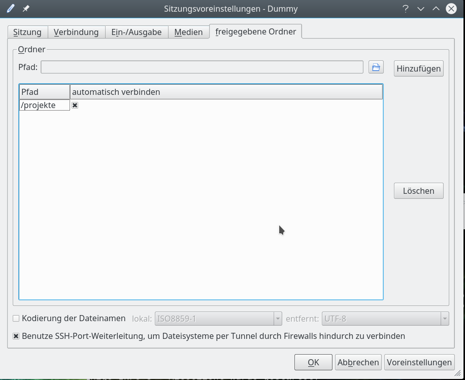
- Freigabe lokaler Verzeichnisse: X2Go erlaubt vom Remote-Desktop aus auch einen Zugriff auf (dafür freigegebene) lokale Verzeichnispfade des Arbeitsplatz-PCs. Damit können Files auf dem Remote-Host z.B. in einem graphischen File-Manager zwischen den dortigen Verzeichnissen (des Hosts) und dem lokalen Verzeichnis des Arbeitsplatz-PCs verschoben/kopiert werden. Zur Wahrung der Sicherheit bei solchen Transaktionen gibt es die Option, den Datenaustausch über SSH getunnelt durchzuführen.
- Mehrere Sitzungen gleichzeitig: Will man mehrere Sitzungen zu verschiedenen Servern gleichzeitig öffnen, so startet man auf dem lokalen PC mit “x2goclient &” einfach einen neuen Client. Auch zwei Sitzungen unter unterschiedlichen Benutzernamen zum gleichen Server sind möglich. Ebenso zwei Sitzungen mit derselben Remote-UID für verschiedene Desktops/Window-Manager – z.B. eine Sitzung mit LXDE und eine mit KDE für ein und denselben User auf demselben Remote-Host. X2Go-Client zeigt einem eine Liste laufender Sitzungen und fragt, was mit den laufenden Sitzungen passieren soll. Die lässt man weiterlaufen und wählt für die neue Sitzung die Option “Neu”. Die verschiedenen Remote-Sitzungen zum gleichen Remote-Host teilen sich dann aber natürlich dessen Netzwerk-Ressourcen. Die sind bei Stratos vServern durchaus begrenzt.
- Seamless Mode: X2Go erlaubt anstelle der Anzeige eines kompletten Remote-Desktops theoretisch auch das Remote-Starten einer einzelnen Anwendung und deren Anzeige auf dem lokalen Desktop des Arbeitsplatz-PCs. (Seamless Mode; das Ganze entspricht dann in der klassischen SSH-Welt in etwa dem vorkonfigurierten Aufruf einer grafischen Remote-Applikation nach einem ssh -X.). Leider klappt das aber auf einem KDE5-Plasma-Desktop (s.u.) nicht wie erwartet.
- Desktop-Sharing: X2Go bietet auch die Möglichkeit des Desktop-Sharings zwischen verschiedenen Nutzern an – das habe ich aber unter den Bedingungen eines vServers aber noch nicht ausprobiert. Ich gehe darauf in diesem Artikel auch nicht weiter ein.
Mit jedem dieser Punkte kann ja jeder mal selber herumexperimentieren. Siehe zur Thematik paralleler Sitzungen auch
https://gist.github.com/ ledeuns/ f0612fb43b967c129c88)
Bzgl. des Desktop-Sharings:
http://wiki.x2go.org/ doku.php/ doc:usage:desktop-sharing
Arbeitet man gleichzeitig unter derselben UID mit 2 getrennten Sessions – z.B. einer LXDE- und einer KDE-Sitzung – auf demselben Arbeitsplatz-PC, so können dabei interessante Effekte z.B. unter Libreoffice auftreten: Ist Libreoffice bereits auf einem der (Remote-)Desktops (z.B. dem KDE-Desktop) geöffnet, so wird ein nachfolgendes Libreoffice-Programm, das in einer parallel laufenden LXDE-Sitzung gestartet wird, trotzdem im KDE-Desktop angezeigt. Ansonsten läuft das Meiste aber normal und erwartungsgemäß.
Für mich war wirklich überraschend, dass neben meinen Git-GUIs auch stark grafiklastige Anwendungen wie Libre-Office Draw, Impress, Inkscape etc. gleichzeitig und sehr, sehr flüssig nutzbar waren. Aus meiner Sicht ist hier die Performance eines Terminal-Servers gegeben, die im wesentlichen nur durch die Netzanbindung des vServers ans Internet limitiert wird und im getesteten Umfang (4 parallele 1920×1200 Sitzungen) überhaupt nicht durch CPU/RAM des Virtuozzo Containers für unseren vServer [V30 bzw. V40, HP3PAR] begrenzt wurde.
Weil es so schön ist, nun eine Zusammenstellung der wichtigsten Hinweise zur Installation und Inbetriebnahme von X2Go, die ich bei dieser Gelegenheit im Internet aufgesammelt habe.
X2Go-Installation: Passende Repositories ziehen
Unter folgendem Link ist beschrieben, wo man die aktuellen Repositories mit X2Go-Komponenten für Debian 8 (64Bit) findet: http://wiki.x2go.org/ doku.php/ wiki:repositories:debian.
Man trägt dann die Repositories über folgende Zusatzzeilen in die Datei “/etc/apt/sources.list” ein:
root@myremotedebian:~# cat /etc/apt/sources.list
# See sources.list(5) for more information, especialy
# Remember that you can only use http, ftp or file URIs
# CDROMs are managed through the apt-cdrom tool.
deb ftp://ftp.stratoserver.net/pub/linux/debian/ jessie main contrib non-free
deb ftp://ftp.stratoserver.net/pub/linux/debian-security/ jessie/updates main contrib non-free

#ICH - 15.04.2017 - Repos for X2Go:
# -----------------------------------
#X2Go Repo
deb http://packages.x2go.org/debian jessie main
# X2Go Repository (sources of release builds)
deb-src http://packages.x2go.org/debian jessie main
Zur Sicherheit machen wir den zugehörigen Key verfügbar; als root:
root@myremotedebian:~ # apt-key adv --recv-keys --keyserver keys.gnupg.net E1F958385BFE2B6E
Dann Update der Paket-Datenbank durchführen:
root@myremotedebian:~ # apt-get update
Nun – als Test – Installieren des Schlüssels über ein Paket aus dem X2Go-Repository:
root@myremotedebian:~ # apt-get install x2go-keyring && apt-get update
Dann die Pakete x2goserver und x2goserver-xsession installieren:
root@myremotedebian:~ # apt-get install x2goserver
Bei mir wurde x2goserver-xsession automatisch mit installiert. Falls das nicht der Fall sein sollte:
root@myremotedebian:~ # apt-get install x2goserver-xsession
Man glaubt es vielleicht nicht – aber das war es im Prinzip serverseitig schon. Zumindest was X2Go anbelangt. Der Grund hierfür ist, dass der X2GO-Client (s.u.) eine SSH-Sitzung nutzt und im Zuge des SSH-Logins die nötigen Umgebungsvariablen setzt und erforderliche Programme auf dem Server für eine Remote-X-Sitzung startet.
LXDE und KDE 4 installieren
Sollte man LXDE oder KDE 4 unter Debian 8 noch nicht installiert haben, so ist dies über
root@myremotedebian:~ # apt-get install lxde
bzw.
root@myremotedebian:~ # apt-get install kde-standard
möglich.
Will man Remote-Audio nutzen, sollte man ggf. auf dem Remote-Host und auch auf dem Arbeitsplatz-PC Pulseaudio installieren. Für mich ist Sound irrelevant – und Pulseaudio kommt bei mir aus Prinzip nicht auf einen PC-Desktop. Aber das mag ja bei anderen anders sein … 🙂
Natürlich muss auf beiden Systemen SSH bereitstehen ..
Auf dem Debian 8 Remote-Host muss zwingend das Paket “openssh-server” installiert sein. Zudem sollte der Server aus Sicherheitsgründen so konfiguriert sein, dass der SSH-Port verlagert ist, sichere Kex-Algorithmen genutzt und eine Authentifizierung über asymmetrische Keys (hinreichender Länge) durchgeführt wird. Der Zugang sollte ferner durch eine Firewall und weitere Maßnahmen auf bestimmte Clients beschränkt werden. Ich gehe auf die SSH-Server-Konfiguration hier nicht weiter ein. Da wir es hier mit gehosteten Remote-Systemen zu tun haben, gehe ich davon aus, dass der zuständige Admin dieses Metier beherrscht.
Jedenfalls muss auf dem Server ein SSHD-Dämon laufen und bereit sein, Logins über einen in der Firewall für bestimmte Clients geöffneten Port entgegen zu nehmen. X2Go tunnelt später die gesamte Kommunikation zwischen Client und Server durch die SSH-Verbindung. Darum muss man sich nicht mehr selber kümmern; s.u.. Es ist übrigens nicht notwendig, für verschiedene Sitzungen auf ein und demselben Remote-Host mehrere unterschiedliche SSH-Ports zu öffnen.
Installation und Nutzung auf dem Arbeitsplatz-PC (X2Go-Client)
Bzgl. der Client-Installation gilt: Es sind passende Pakete für die Distribution zu finden, die man auf seinem Arbeitsplatz-PC einsetzt. Siehe für Hinweise
http://wiki.x2go.org/ doku.php/ doc:installation: x2goclient.
Ich beschreibe die Clientseite hier nur für einen Opensuse Leap 42.2 Client. Für Opensuse liegen die erforderlichen RPMs unter folgendem Repository:
repositories/X11:/RemoteDesktop:/ x2go/openSUSE_Leap_42.2/
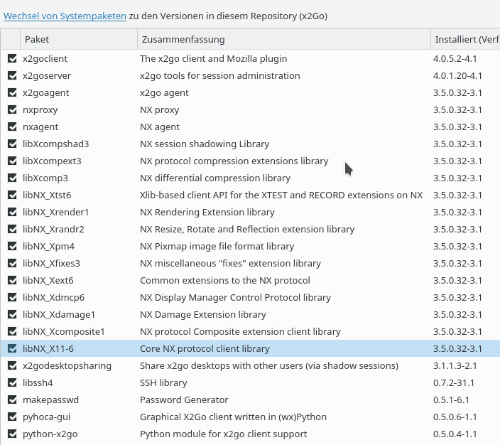
Von dort installiert man mittels YaST etwa “x2goclient”, “pyhoca-gui”. Der Rest der benötigten Pakete wird dann über Abhängigkeiten nachgezogen:
Nun öffnet man auf seinem Client-PC den Client am Terminal etwa über:
ich@mytux:~> x2goclient &
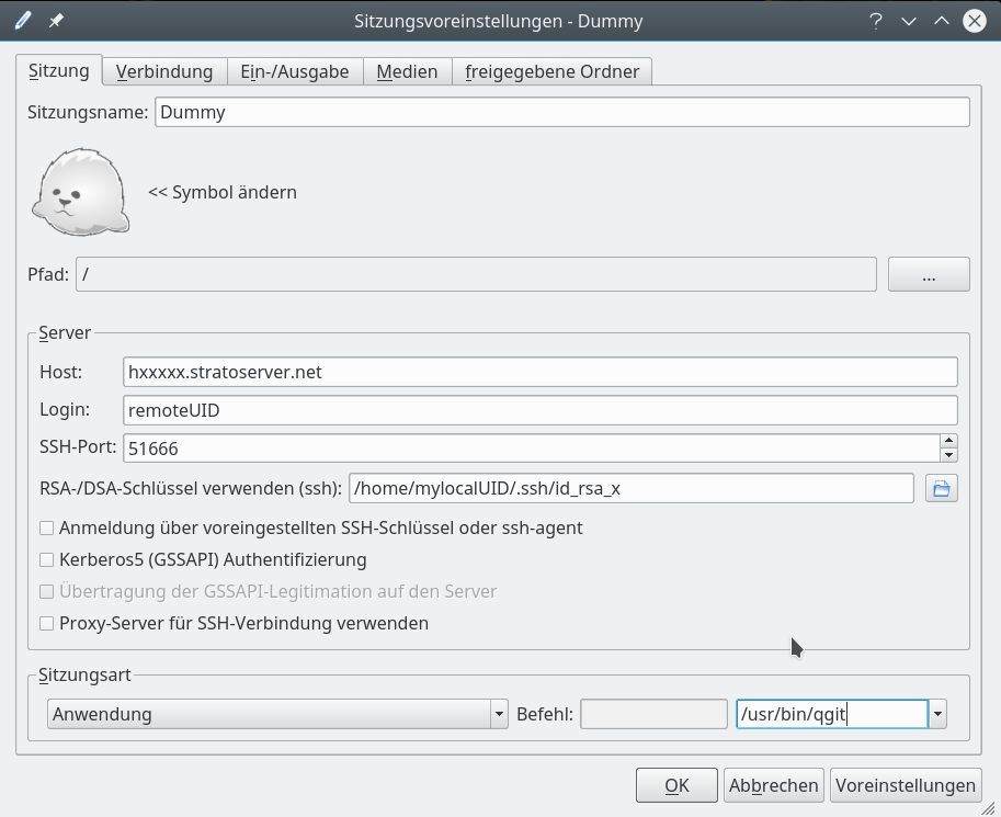
Es öffnet sich initial eine Oberfläche, die die Anlage von sog. “Sitzungen” zu Remote-Hosts erlaubt; diese “Sitzungsvarianten” werden später im X2Go-Client-Fenster zur Auswahl angeboten.
Ich zeige nachfolgende die verschiedenen Konfigurationsdialoge für eine Sitzung (die ich “Dummy” genannt habe). Natürlich muss man die Eingabefelder mit den für seine eigene Situation passenden Daten ausfüllen.
Siehe für eine ausführliche Beschreibung des X2Go-Client-Setups zudem:
http://wiki.x2go.org/ doku.php/ doc:usage:x2goclient
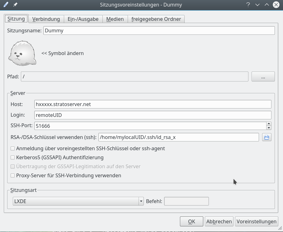
Zunächst – und das ist das Wichtigste – müssen wir die Serververbindung einstellen:
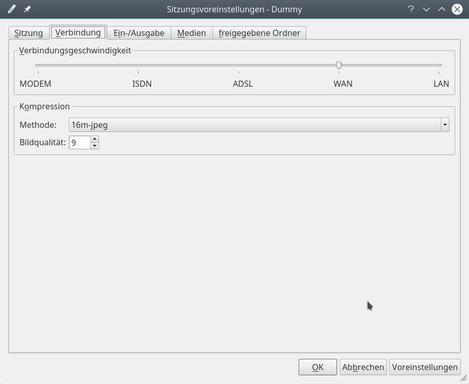
Dann steht eine Konfiguration der Bandbreite der Verbindung an:
Wir wenden uns anschließend einer Konfiguration der Auflösung der Desktop-Darstellung zu:
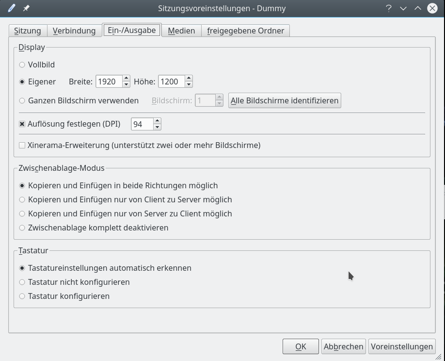
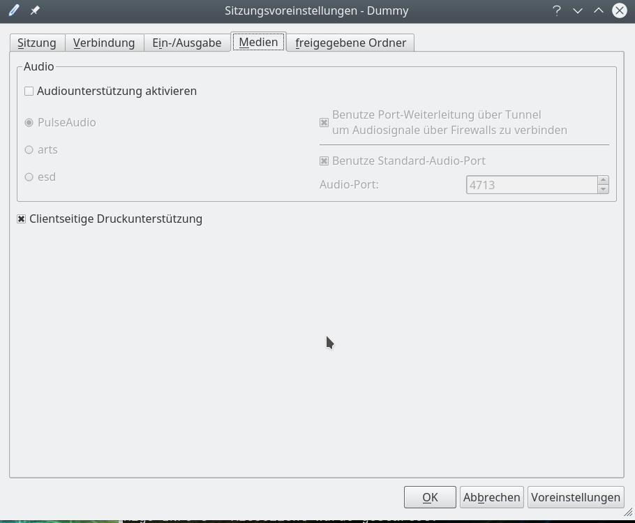
Für erste Tests deaktivieren mal die Sound-Unterstützung:
Als letztes kann man konfigurieren, ob man bestimmte Verzeichnisse auf dem Arbeitsplatz-PCs für einen direkten Zugriff durch Remote_X-Client-Programme freigeben will. Tut man das, so sollte man in jedem Fall die zugehörige Option zur SSH-Port-Weiterleitung aktivieren.
Man kann all diese Konfigurationseinstellungen später über den Menüpunkt “Sitzung => Sitzungsverwaltung” nachbessern.
Resultate
Hat man seine “Sitzung” konfiguriert, so steht diese im rechten Bereich des X2Go-Client-Fensters zur Aktivierung bereit.
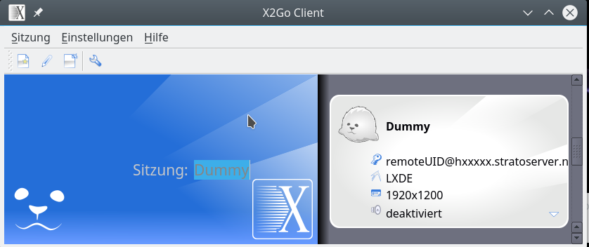
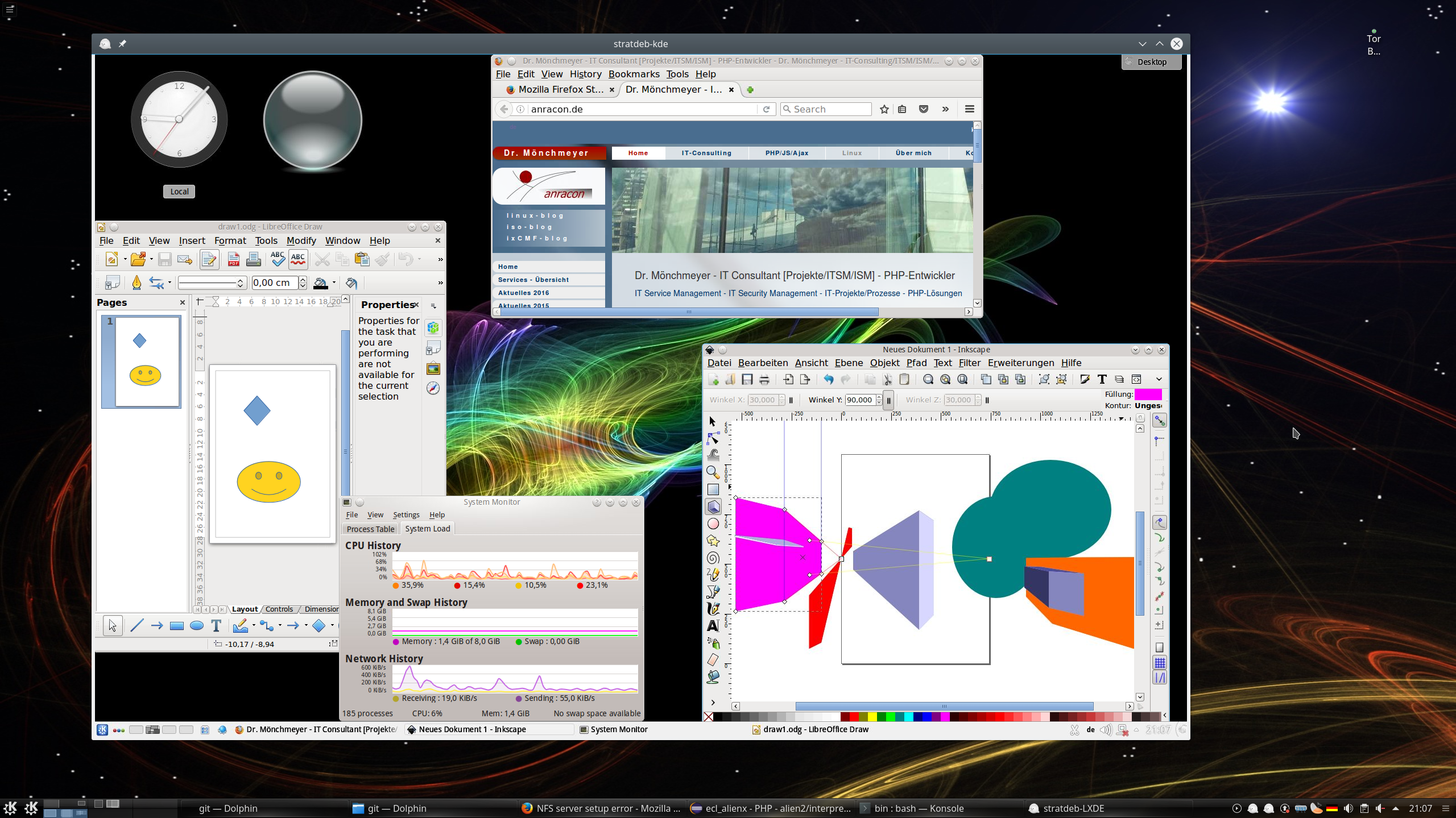
Nach einem Doppelklick rückt die aktivierte Verbindung ins Zentrum der Anzeige; in unserem Fall öfnnet sich zudem ein kleines Dialogfenster, in dem wir die Passphrase für unseren SSH-Key eingeben müssen. Und nach wenigen Augenblicken/Sekunden öffnet sich schließlich das Fenster für unseren Remote-Desktop – hier mit LXDE :
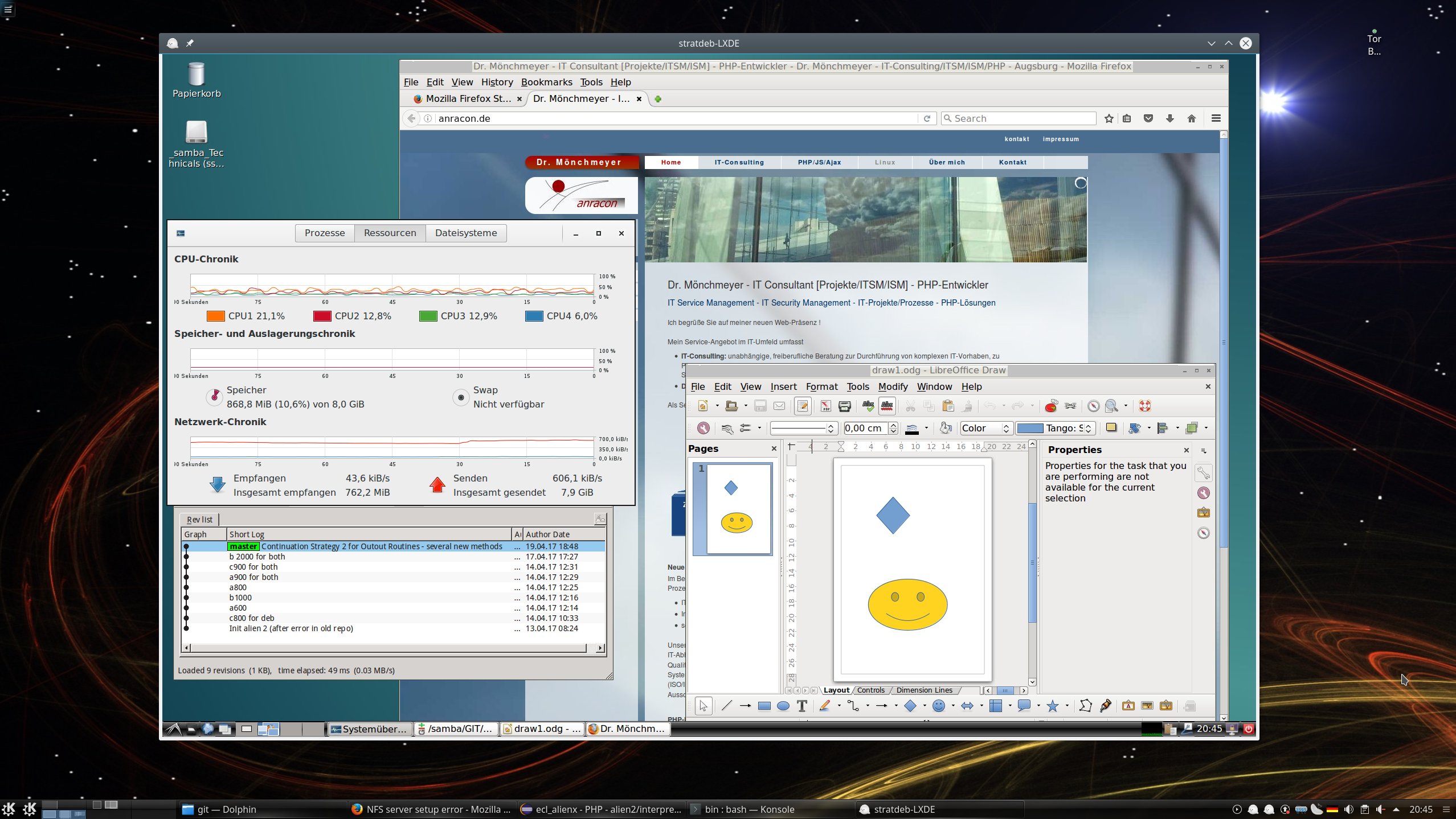
Der aufmerksame Betrachter wird Qgit im linken Bildbereich entdeckt haben – hier für ein noch sehr langweiliges Test-Repository. Ich habe fast alle mir unter Linux bekannten Git-Clients ausprobiert – jeder läuft flüssig; fast wie lokal.
Das Ganze nun auch nochmal für einen Remote-KDE-Desktop:
Für 2 parallele Sitzungen zum gleichen Server muss man einfach zwei x2go-Clients öffnen und in einer zwischenzeitlichen Anzeige bereits geöffneter Sessions die Optionen so wählen, dass die bereits geöffnete Sitzung nicht unterbrochen werden soll, sondern dass eine neue Sitzung geöffnet werden soll.
Die nachfolgende Abbildung zeigt zwei parallel zu einem vServer unter Debian 8 geöffnete Sitzungen – eine unter LXDE, die andere unter KDE4:
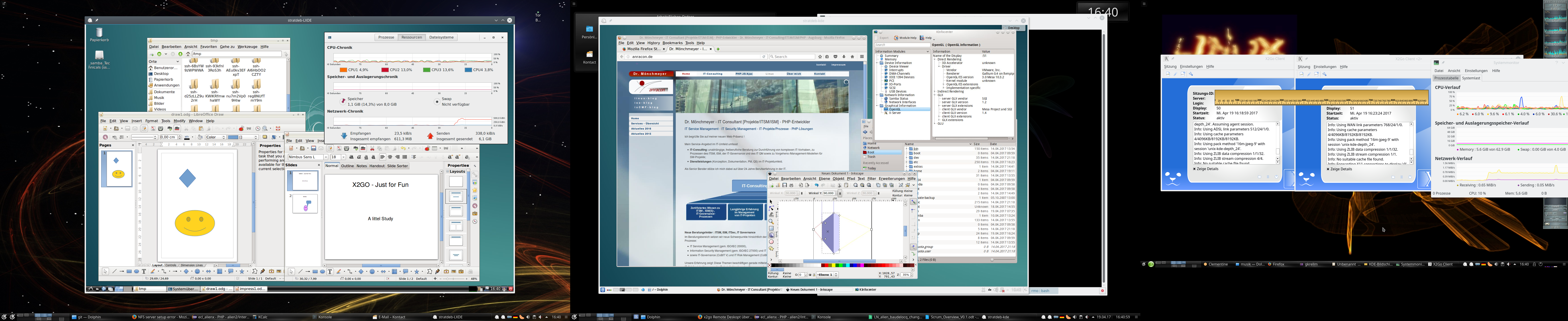
Getestet habe ich das Ganze mit einer vDSL-Leitung, aber auch einer ADSL-16MBit-Leitung – auch bei letzterer sind mehrere gleichzeitige Sitzungen kein Problem !
Wo so viel Licht ist, gibt es aber auch Schatten. Daher sei abschließend noch auf 2 Punkte hingewiesen, die in der Praxis relevant werden können.
Problematischer Punkt bzgl. der Soundunterstützung und Firefox unter X2Go
Im Prinzip kann X2Go (angeblich) Audio-Daten übertragen. Allerdings über einen Pulseaudio-Server. Den habe ich bei mir allerdings wegen vieler Probleme mit einer Xonar D2X und einer X-Fi nicht am Laufen. Ich benutze ausschließlich plain Alsa – das funktioniert zuverlässig und erlaubt das Umschiffen vieler Pulseaudio-Probleme. Fakt ist jedenfalls, dass es mit einer aktivierten Sound-Unterstützung für Pulseaudio unter X2Go und einem remote gestarteten Firefox ESR erhebliche Probleme gibt:
Alle Menüpunkte der Firefox-Oberfläche reagieren nicht mehr bzw. mit erheblicher (!) Zeitverzögerung auf Maus-Klicks im X2GO-Client. Firefox wirkt wie eingefroren; das stimmt aber nicht – die Reaktion kommt nur mit Minuten Verzögerung. Das ist u.a. hier beschrieben:
http://thescriptingadmin.blogspot.de/ 2015/09/ firefox-freezing-on-linux-x2go.html
https://debianforum.de/ forum/ viewtopic.php?t=164257
Wer immer daran Schuld hat. Da das mit anderen GTK-Anwendungen als FF nicht passiert, tippe ich darauf, dass FF bei installiertem PA auch erwartet, dass PA reagiert. Was remote evtl. ein Problem darstellt, wenn dort PA ggf. gar nicht installiert ist.
Ich habe mangels Interesse nicht getestet, ob dieser Fehler u.U. daran liegt, dass auf meinem Arbeitsplatz PA nicht aktiv ist. Lasst mir gerne eine Email zukommen, wenn ihr dazu was wisst. Ich persönlich verzichte aber lieber auf Sound von einer Remote-X2Go-Quelle, als mich mit PA herumzuschlagen. Vielleicht probiere ich das später mal auf einem Laptop. Falls ihr auch auf dieses Problem mit FF stoßen solltet und bereit seid, auf Sound vom X2go-Server zu verzichten, gilt Folgendes:
Wichtiger Hinweis zu einem Problem mit Firefox und dem X2Go-Client unter Linux:
Soundunterstützung im X2Go-Client abschalten (Reiter “Medien” unter den Einstellungen) oder aber auf einen anderen Soundserver umschalten. Bei mir funktionierte ein Remote-Firefox FF im X2Go-Desktop-Fenster nach einer Abschaltung der Soundunterstützung durch Pulseaudio problemfrei.
X2Go Seamless Mode funktioniert nicht unter KDE5
X2Go bietet zwar im Prinzip die Möglichkeit an, Remote X-Anwendungen auch als singuläre Applikationen zu starten, die direkt als Fenster (also ohne umgebenden Remote-Desktop) in den Desktop des Arbeitsplatz-PCs eingeblendet werden.
Hierzu konfiguriert man eine entsprechende Sitzung, z.B. nur für “qgit”, wie folgt:
Danach startet die angegebene Applikation im seamless Fenstermode. Das klappt auch mit einem Terminal wie etwa “lxterminal” (“/usr/bin/lxterminal”). Von der Kommandozeile aus, kann man dann weitere Anwendungen wie “qgit” starten, die dann wiederum als Einzelapplikation auf dem lokalen Desktop angezeigt werden.
Leider täuscht aber der erste positive Eindruck; unter KDE5 sind die zugehörigen Fenster für komplexere Anwendungen als ein Terminal in ihrer Größe leider nicht veränderbar. Das macht den Einsatz des “Seamless Mode” für KDE5 am Arbeitsplatz-PC in der Praxis unbrauchbar. Der seamless Mode funktioniert aber sehr wohl unter einem LXDE-Desktop am Arbeitsplatz-PC.
Fazit
X2Go bietet eine einfache zu handhabende Möglichkeit, performant von einem Linux-Arbeitsplatz-PC auf grafische Anwendungen eines Remote-Strato-vServers zuzugreifen. Die Linux-Installation des vServers muss lediglich einen LXDE- oder KDE4-Desktop unterstützen. (Desktops unter XFCE, Mate, LXQT habe ich nicht getestet; das sollte aber auch alles funktionieren).
Als einzige Wermutstropfen bleiben, dass der Seamless Mode auf einem KDE5-Target-Desktop des Arbeitsplatz-PCs nicht richtig funktioniert und dass im Moment weder native KDE5- noch Gnome3-Desktops des vServers unterstützt werden. Angeblich wird daran aber bereits von den X2Go-Entwicklern gearbeitet; wir freuen uns auf entsprechende neue X2Go-Versionen.
Links
Was ist X2GO?
http://www.mn.uio.no/geo/ english/services/it/help/ using-linux/x2go.html
https://de.wikipedia.org/ wiki/ NX_NoMachine
http://xmodulo.com/x2go-remote-desktop-linux.html
https://serverfault.com/ questions/227542/ what-alternatives-to-vnc-are-there-for-linux
Details zum Server
http://wiki.x2go.org/doku.php/wiki: advanced: x2goserver-in-detail
Installation von X2Go
http://wiki.x2go.org/doku.php/ wiki:repositories:debian
https://www.sugar-camp.com/x2go-vorstellung-und-installationsanleitung/
http://wiki.x2go.org/ doku.php/ doc:installation:x2goserver
http://www.linux-community.de/Internal/Artikel/ Print-Artikel/LinuxUser/2011/07/X2go-Terminalserver-auch-fuer-den-Hausgebrauch
http://xmodulo.com/x2go-remote-desktop-linux.html
https://mun-steiner.de/ wordpress/ index.php/ linux/ x2go-mit-ssh/
https://wiki.archlinux.de/title/X2go
Installation und Übersicht über ein paar Bugs
http://www.mn.uio.no/geo/english/ services/it/help/ using-linux/x2go.html
VNC : Benötigt VNC einen X-Server?
https://unix.stackexchange.com/ questions/ 129432/vnc-server-without-x-window-system

