A simple Python program for an ANN to cover the MNIST dataset – III – forward propagation

I continue with my efforts of writing a small Python class by which I can setup and test a Multilayer Perceptron [MLP] as a simple example for an artificial neural network [ANN]. In the last two articles of this series

A simple program for an ANN to cover the Mnist dataset – II – initial random weight values
A simple program for an ANN to cover the Mnist dataset – I – a starting point

I defined some code elements, which controlled the layers, their node numbers and built weight matrices. We succeeded in setting random initial values for the weights. This enables us to work on the forward propagation algorithm in this article.

Methods to cover training and mini-batches

As we later on need to define methods which cover “training epochs” and the handling of “mini-batches” comprising a defined number of training records we extend our set of methods already now by

An “epoch” characterizes a full training step comprising

  • propagation, cost and derivative analysis and weight correction of all data records or samples in the set of training data, i.e. a loop over all mini-batches.

Handling of a mini-batch comprises

  • (vectorized) propagation of all training records of a mini-batch,
  • cumulative cost analysis for all training records of a batch,
  • cumulative, averaged gradient evaluation of the cost function by back-propagation of errors and summation over all records of a training batch,
  • weight corrections for nodes in all layers based on averaged gradients over all records of the batch data.

Vectorized propagation means that we propagate all training records of a batch in parallel. This will be handled by Numpy matrix multiplications (see below).
We shall see in a forthcoming that we can also cover the cumulative gradient calculation over all batch samples by matrix-multiplications where we shift the central multiplication and summation operations to appropriate rows and columns.

However, we do not care for details of training epochs and complete batch-operations at the moment. We use the two methods “_fit()” and “_handle_mini_batch()” in this article only as envelopes to trigger the epoch loop and the matrix operations for propagation of a batch, respectively.

Modified “__init__”-function

We change and extend our “__init_”-function of class MyANN a bit:

    def __init__(self, 
                 my_data_set = "mnist", 
                 n_hidden_layers = 1, 
                 ay_nodes_layers = [0, 100, 0], # array which should have as much elements as n_hidden + 2
                 n_nodes_layer_out = 10,  # expected number of nodes in output layer 
                                                  
                 my_activation_function = "sigmoid", 
                 my_out_function        = "sigmoid",   
                 
                 n_size_mini_batch = 50,  # number of data elements in a mini-batch 
                 
                 n_epochs      = 1,
                 n_max_batches = -1,  # number of mini-batches to use during epochs - > 0 only for testing 
                                      # a negative value uses all mini-batches 
                 
                 vect_mode = 'cols', 
                 
                 figs_x1=12.0, figs_x2=8.0, 
                 legend_loc='upper right',
                 
n                 b_print_test_data = True
                 
                 ):
        '''
        Initialization of MyANN
        Input: 
            data_set: type of dataset; so far only the "mnist", "mnist_784" datsets are known 
                      We use this information to prepare the input data and learn about the feature dimension. 
                      This info is used in preparing the size of the input layer.     
            n_hidden_layers = number of hidden layers => between input layer 0 and output layer n 

            ay_nodes_layers = [0, 100, 0 ] : We set the number of nodes in input layer_0 and the output_layer to zero 
                              Will be set to real number afterwards by infos from the input dataset. 
                              All other numbers are used for the node numbers of the hidden layers.
            n_nodes_out_layer = expected number of nodes in the output layer (is checked); 
                                this number corresponds to the number of categories NC = number of labels to be distinguished
            
            my_activation_function : name of the activation function to use 
            my_out_function : name of the "activation" function of the last layer which produces the output values 
            
            n_size_mini_batch : Number of elements/samples in a mini-batch of training data 
                                The number of mini-batches will be calculated from this
            
            n_epochs : number of epochs to calculate during training
            n_max_batches : > 0: maximum of mini-batches to use during training 
                            < 0: use all mini-batches  
            
            vect_mode: Are 1-dim data arrays (vctors) ordered by columns or rows ?

            figs_x1=12.0, figs_x2=8.0 : Standard sizing of plots , 
            legend_loc='upper right': Position of legends in the plots
            
            b_print_test_data: Boolean variable to control the print out of some tests data 
             
         '''
        
        # Array (Python list) of known input data sets 
        self._input_data_sets = ["mnist", "mnist_784", "mnist_keras"]  
        self._my_data_set = my_data_set
        
        # X, y, X_train, y_train, X_test, y_test  
            # will be set by analyze_input_data 
            # X: Input array (2D) - at present status of MNIST image data, only.    
            # y: result (=classification data) [digits represent categories in the case of Mnist]
        self._X       = None 
        self._X_train = None 
        self._X_test  = None   
        self._y       = None 
        self._y_train = None 
        self._y_test  = None
        
        # relevant dimensions 
        # from input data information;  will be set in handle_input_data()
        self._dim_sets     = 0  
        self._dim_features = 0  
        self._n_labels     = 0   # number of unique labels - will be extracted from y-data 
        
        # Img sizes 
        self._dim_img      = 0 # should be sqrt(dim_features) - we assume square like images  
        self._img_h        = 0 
        self._img_w        = 0 
        
        # Layers
        # ------
        # number of hidden layers 
        self._n_hidden_layers = n_hidden_layers
        # Number of total layers 
        self._n_total_layers = 2 + self._n_hidden_layers  
        # Nodes for hidden layers 
        self._ay_nodes_layers = np.array(ay_nodes_layers)
        # Number of nodes in output layer - will be checked against information from target arrays
        self._n_nodes_layer_out = n_nodes_layer_out
        
        
        # Weights 
        # --------
        # empty List for all weight-matrices for all layer-connections
        # Numbering : 
        # w[0] contains the weight matrix 
which connects layer 0 (input layer ) to hidden layer 1 
        # w[1] contains the weight matrix which connects layer 1 (input layer ) to (hidden?) layer 2 
        self._ay_w = []  
        
        # --- New -----
        # Two lists for output of propagation
        # __ay_x_in  : input data of mini-batches on the different layers; the contents is calculated by the propagation algorithm    
        # __ay_a_out : output data of the activation function; the contents is calculated by the propagation algorithm
        # Note that the elements of these lists are numpy arrays     
        self.__ay_X_in  = []  
        self.__ay_a_out = [] 
        
        
        # Known Randomizer methods ( 0: np.random.randint, 1: np.random.uniform )  
        # ------------------
        self.__ay_known_randomizers = [0, 1]

        # Types of activation functions and output functions 
        # ------------------
        self.__ay_activation_functions = ["sigmoid"] # later also relu 
        self.__ay_output_functions     = ["sigmoid"] # later also softmax 
        
        # the following dictionaries will be used for indirect function calls 
        self.__d_activation_funcs = {
            'sigmoid': self._sigmoid, 
            'relu':    self._relu
            }
        self.__d_output_funcs = { 
            'sigmoid': self._sigmoid, 
            'softmax': self._softmax
            }  
          
        # The following variables will later be set by _check_and set_activation_and_out_functions()            
        self._my_act_func = my_activation_function
        self._my_out_func = my_out_function
        self._act_func = None    
        self._out_func = None    

        # number of data samples in a mini-batch 
        self._n_size_mini_batch = n_size_mini_batch
        self._n_mini_batches = None  # will be determined by _get_number_of_mini_batches()

        # number of epochs 
        self._n_epochs = n_epochs
        # maximum number of batches to handle (<0 => all!) 
        self._n_max_batches = n_max_batches


        # print some test data 
        self._b_print_test_data = b_print_test_data

        # Plot handling 
        # --------------
        # Alternatives to resize plots 
        # 1: just resize figure  2: resize plus create subplots() [figure + axes] 
        self._plot_resize_alternative = 1 
        # Plot-sizing
        self._figs_x1 = figs_x1
        self._figs_x2 = figs_x2
        self._fig = None
        self._ax  = None 
        # alternative 2 does resizing and (!) subplots() 
        self.initiate_and_resize_plot(self._plot_resize_alternative)        
        
        
        # ***********
        # operations 
        # ***********
        
        # check and handle input data 
        self._handle_input_data()
        # set the ANN structure 
        self._set_ANN_structure()
        
        # Prepare epoch and batch-handling - sets mini-batch index array, too 
        self._prepare_epochs_and_batches()
        
        # perform training 
        start_c = time.perf_counter()
        self._fit(b_print=True, b_measure_batch_time=False)
        end_c = time.perf_counter()
        print('\n\n ------') 
        print('Total training Time_CPU: ', end_c - start_c) 
        print("\nStopping program regularily")
        sys.exit()

 
Readers who have followed me so far will recognize that I renamed the parameter “n_mini_batch” to “n_size_mini_batch” to indicate its purpose a bit more clearly. We shall derive the number of required mini-batches form the value of this parameter.
I have added two new parameters:

  • n_epochs = 1
  • n_max_batches = -1

“n_epochs” will later receive the user’s setting for the number of epochs to
follow during training. “n_max_Batches” allows us to limit the number of mini-batches to analyze during tests.

The kind reader will also have noticed that I encapsulated the series of operations for preparing the weight-matrices for the ANN in a new method “_set_ANN_structure()

    
    '''-- Main method to set ANN structure --''' 
    def _set_ANN_structure(self):
        # check consistency of the node-number list with the number of hidden layers (n_hidden)
        self._check_layer_and_node_numbers()
        # set node numbers for the input layer and the output layer
        self._set_nodes_for_input_output_layers() 
        self._show_node_numbers() 

        # create the weight matrix between input and first hidden layer 
        self._create_WM_Input() 
        # create weight matrices between the hidden layers and between tha last hidden and the output layer 
        self._create_WM_Hidden() 

        # check and set activation functions 
        self._check_and_set_activation_and_out_functions()
        
        return None

 
The called functions have remained unchanged in comparison to the last article.

Preparing epochs and batches

We can safely assume that some steps must be performed to prepare epoch- and batch handling. We, therefore, introduced a new function “_prepare_epochs_and_batches()”. For the time being this method only calculates the number of mini-batches from the input parameter “n_size_mini_batch”. We use the Numpy-function “array_split()” to split the full range of input data into batches.

 
    ''' -- Main Method to prepare epochs -- '''
    def _prepare_epochs_and_batches(self):
        # set number of mini-batches and array with indices of input data sets belonging to a batch 
        self._set_mini_batches()
        return None
##    
    ''' -- Method to set the number of batches based on given batch size -- '''
    def _set_mini_batches(self, variant=0): 
        # number of mini-batches? 
        self._n_mini_batches = math.ceil( self._y_train.shape[0] / self._n_size_mini_batch )
        print("num of mini_batches = " + str(self._n_mini_batches))
        
        # create list of arrays with indices of batch elements 
        self._ay_mini_batches = np.array_split( range(self._y_train.shape[0]), self._n_mini_batches )
        print("\nnumber of batches : " + str(len(self._ay_mini_batches)))
        print("length of first batch : " + str(len(self._ay_mini_batches[0])))
        print("length of last batch : "  + str(len(self._ay_mini_batches[self._n_mini_batches - 1]) ))
        return None

 
Note that the approach may lead to smaller batch sizes than requested by the user.
array_split() cuts out a series of sub-arrays of indices of the training data. I.e., “_ay_mini_batches” becomes a 1-dim array, whose elements are 1-dim arrays, too. Each of the latter contains a collection of indices for selected samples of the training data – namely the indices for those samples which shall be used in the related mini-batch.

Preliminary elements of the method for training – “_fit()”

For the time being method “_fit()” is used for looping over the number of epochs and the number of batches:

 
    ''' -- Method to set the number of batches based on given batch size -- '''
    def _fit(self, b_print = False, b_measure_batch_time = False):
        # range of epochs
        ay_idx_epochs  = range(0, self._n_epochs)
        
        # limit the number of mini-batches
        n_max_batches = min(self._n_max_
batches, self._n_mini_batches)
        ay_idx_batches = range(0, n_max_batches)
        if (b_print):
            print("\nnumber of epochs = " + str(len(ay_idx_epochs)))
            print("max number of batches = " + str(len(ay_idx_batches)))
        
        # looping over epochs
        for idxe in ay_idx_epochs:
            if (b_print):
                print("\n ---------")
                print("\nStarting epoch " + str(idxe+1))
            
            # loop over mini-batches
            for idxb in ay_idx_batches:
                if (b_print):
                    print("\n ---------")
                    print("\n Dealing with mini-batch " + str(idxb+1))
                if b_measure_batch_time: 
                    start_0 = time.perf_counter()
                # deal with a mini-batch
                self._handle_mini_batch(num_batch = idxb, b_print_y_vals = False, b_print = b_print)
                if b_measure_batch_time: 
                    end_0 = time.perf_counter()
                    print('Time_CPU for batch ' + str(idxb+1), end_0 - start_0) 
        
        return None
#

 
We limit the number of mini_batches. The double-loop-structure is typical. We tell function “_handle_mini_batch(num_batch = idxb,…)” which batch it should handle.

Preliminary steps for the treatment of a mini-batch

We shall build up the operations for batch handling over several articles. In this article we clarify the operations for feed forward propagation, only. Nevertheless, we have to think a step ahead: Gradient calculation will require that we keep the results of propagation layer-wise somewhere.

As the number of layers can be set by the user of the class we save the propagation results in two Python lists:

  • ay_Z_in_layer = []
  • ay_A_out_layer = []

The Z-values define a collection of input vectors which we normally get by a matrix multiplication from output data of the last layer and a suitable weight-matrix. The “collection” is our mini-batch. So, “ay_Z_in_layer” actually is a 2-dimensional array.

For the ANN’s input layer “L0”, however, we just fill in an excerpt of the “_X”-array-data corresponding to the present mini-batch.

Array “ay_A_out_layer[n]” contains the results of activation function applied onto the elements of “ay_Z_in_layer[n]” of Layer “Ln”. (In addition we shall add a value for a bias neutron; see below).

Our method looks like:

 
    ''' -- Method to deal with a batch -- '''
    def _handle_mini_batch(self, num_batch = 0, b_print_y_vals = False, b_print = False):
        '''
        For each batch we keep the input data array Z and the output data A (output of activation function!) 
        for all layers in Python lists
        We can use this as input variables in function calls - mutable variables are handled by reference values !
        We receive the A and Z data from propagation functions and proceed them to cost and gradient calculation functions
        
        As an initial step we define the Python lists ay_Z_in_layer and ay_A_out_layer 
        and fill in the first input elements for layer L0  
        '''
        ay_Z_in_layer  = [] # Input vector in layer L0;  result of a matrix operation in L1,...
        ay_A_out_layer = [] # Result of activation function 
    
        #print("num_batch = " + str(num_batch))
        #print("len of ay_mini_batches = " + str(len(self._ay_mini_batches))) 
        #print("_ay_mini_batches[0] = ")
        #print(self._ay_mini_batches[num_batch])
    
        # Step 1: Special treatment of the ANN's input Layer L0
        # Layer L0: Fill in the input vector for the ANN's input layer L0 
       
 ay_Z_in_layer.append( self._X_train[(self._ay_mini_batches[num_batch])] ) # numpy arrays can be indexed by an array of integers
        #print("\nPropagation : Shape of X_in = ay_Z_in_layer = " + str(ay_Z_in_layer[0].shape))           
        if b_print_y_vals:
            print("\n idx, expected y_value of Layer L0-input :")           
            for idx in self._ay_mini_batches[num_batch]:
                print(str(idx) + ', ' + str(self._y_train[idx]) )
        
        # Step 2: Layer L0: We need to transpose the data of the input layer 
        ay_Z_in_0T       = ay_Z_in_layer[0].T
        ay_Z_in_layer[0] = ay_Z_in_0T

        # Step 3: Call the forward propagation method for the mini-batch data samples 
        self._fw_propagation(ay_Z_in = ay_Z_in_layer, ay_A_out = ay_A_out_layer, b_print = b_print) 
        
        if b_print:
            # index range of layers 
            ilayer = range(0, self._n_total_layers)
            print("\n ---- ")
            print("\nAfter propagation through all layers: ")
            for il in ilayer:
                print("Shape of Z_in of layer L" + str(il) + " = " + str(ay_Z_in_layer[il].shape))
                print("Shape of A_out of layer L" + str(il) + " = " + str(ay_A_out_layer[il].shape))

        
        # Step 4: To be done: cost calculation for the batch 
        # Step 5: To be done: gradient calculation via back propagation of errors 
        # Step 6: Adjustment of weights  
        
        # try to accelerate garbage handling
        if len(ay_Z_in_layer) > 0:
            del ay_Z_in_layer
        if len(ay_A_out_layer) > 0:
            del ay_A_out_layer
        
        return None

 
Why do we need to transpose the Z-matrix for layer L0?
This has to do with the required matrix multiplication of the forward propagation (see below).

The function “_fw_propagation()” performs the forward propagation of a mini-batch through all of the ANN’s layers – and saves the results in the lists defined above.

Important note: We transfer our lists (mutable Python objects) to “_fw_propagation()”! This has the effect that the array of the corresponding values is referenced from within “_fw_propagation()”; therefore will any elements added to the lists also be available outside the called function! Therefore we can use the calculated results also in further functions for e.g. gradient calculations which will later be called from within “_handle_mini_batch()”.

Note also that this function leaves room for optimization: It is e.g. unnecessary to prepare ay_Z_in_0T again and again for each epoch. We will transfer the related steps to “_prepare_epochs_and_batches()” later on.

Forward Propagation

In one of my last articles in this blog I already showed how one can use Numpy’s Linear Algebra features to cover propagation calculations required for information transport between two adjacent layers of a feed forward “Artificial Neural Network” [ANN]:
Numpy matrix multiplication for layers of simple feed forward ANNs

The result was that we can cover propagation between neighboring layers by a vectorized multiplication of two 2-dim matrices – one containing the weights and the other vectors of feature data for all mini-batch samples. In the named article I discussed in detail which rows and columns are used for the central multiplication with weights and summations – and that the last dimension of the input array should account for the mini-batch samples. This requires the transpose operation on the input array of Layer L0. All other intermediate layer results (arrays) do already get the right form for vectorizing.

“_fw_propagation()” takes the following form:

 
    ''' -- Method to handle FW propagation for a mini-batch --'''
    def _fw_propagation(self, ay_Z_in, ay_A_out, b_print= False):
        
        b_internal_timing = False
        
        # index range of layers 
        ilayer = range(0, self._n_total_layers-1)

        # propagation loop
        for il in ilayer:
            if b_internal_timing: start_0 = time.perf_counter()
            
            if b_print: 
                print("\nStarting propagation between L" + str(il) + " and L" + str(il+1))
                print("Shape of Z_in of layer L" + str(il) + " (without bias) = " + str(ay_Z_in[il].shape))
            
            # Step 1: Take input of last layer and apply activation function 
            if il == 0: 
                A_out_il = ay_Z_in[il] # L0: activation function is identity 
            else: 
                A_out_il = self._act_func( ay_Z_in[il] ) # use real activation function 
            
            # Step 2: Add bias node 
            A_out_il = self._add_bias_neuron_to_layer(A_out_il, 'row')
            # save in array     
            ay_A_out.append(A_out_il)
            if b_print: 
                print("Shape of A_out of layer L" + str(il) + " (with bias) = " + str(ay_A_out[il].shape))
            
            # Step 3: Propagate by matrix operation 
            Z_in_ilp1 = np.dot(self._ay_w[il], A_out_il) 
            ay_Z_in.append(Z_in_ilp1)
            
            if b_internal_timing: 
                end_0 = time.perf_counter()
                print('Time_CPU for layer propagation L' + str(il) + ' to L' + str(il+1), end_0 - start_0) 
        
        # treatment of the last layer 
        il = il + 1
        if b_print:
            print("\nShape of Z_in of layer L" + str(il) + " = " + str(ay_Z_in[il].shape))
        A_out_il = self._out_func( ay_Z_in[il] ) # use the output function 
        ay_A_out.append(A_out_il)
        if b_print:
            print("Shape of A_out of last layer L" + str(il) + " = " + str(ay_A_out[il].shape))
        
        return None
#

 
First we set a range for a loop over the layers. Then we apply the activation function. In “step 2” we add a bias-node to the layer – compare this to the number of weights, which we used during the initialization of the weight matrices in the last article. In step 3 we apply the vectorized Numpy-matrix multiplication (np.dot-operation). Note that this is working for layer L0, too, because we already transposed the input array for this layer in “_handle_mini_batch()”!

Note that we need some special treatment for the last layer: here we call the out-function to get result values. And, of course, we do not add a bias neuron!

It remains to have a look at the function “_add_bias_neuron_to_layer(A_out_il, ‘row’)”, which extends the A-data by a constant value of “1” for a bias neuron. The function is pretty simple:

    ''' Method to add values for a bias neuron to A_out '''
    def _add_bias_neuron_to_layer(self, A, how='column'):
        if how == 'column':
            A_new = np.ones((A.shape[0], A.shape[1]+1))
            A_new[:, 1:] = A
        elif how == 'row':
            A_new = np.ones((A.shape[0]+1, A.shape[1]))
            A_new[1:, :] = A
        return A_new    

A first test

We let the program run in a Jupyter cell with the following parameters:

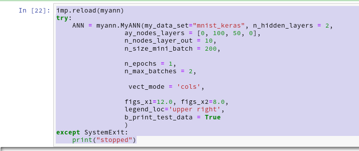
This produces the following output ( I omitted the output for initialization):

 
Input data for dataset mnist_keras : 
Original shape of X_train = (60000, 28, 28)
Original Shape of y_train = (60000,)
Original shape of X_test = (10000, 28, 28)
Original Shape of y_test = (10000,)

Final input data for dataset mnist_keras : 
Shape of X_train = (60000, 784)
Shape of y_train = (60000,)
Shape of X_test = (10000, 784)
Shape of y_test = (10000,)

We have 60000 data sets for training
Feature dimension is 784 (= 28x28)
The number of labels is 10

Shape of y_train = (60000,)
Shape of ay_onehot = (10, 60000)

Values of the enumerate structure for the first 12 elements : 
(0, 6)
(1, 8)
(2, 4)
(3, 8)
(4, 6)
(5, 5)
(6, 9)
(7, 1)
(8, 3)
(9, 8)
(10, 9)
(11, 0)

Labels for the first 12 datasets:

Shape of ay_onehot = (10, 60000)
[[0. 0. 0. 0. 0. 0. 0. 0. 0. 0. 0. 1.]
 [0. 0. 0. 0. 0. 0. 0. 1. 0. 0. 0. 0.]
 [0. 0. 0. 0. 0. 0. 0. 0. 0. 0. 0. 0.]
 [0. 0. 0. 0. 0. 0. 0. 0. 1. 0. 0. 0.]
 [0. 0. 1. 0. 0. 0. 0. 0. 0. 0. 0. 0.]
 [0. 0. 0. 0. 0. 1. 0. 0. 0. 0. 0. 0.]
 [1. 0. 0. 0. 1. 0. 0. 0. 0. 0. 0. 0.]
 [0. 0. 0. 0. 0. 0. 0. 0. 0. 0. 0. 0.]
 [0. 1. 0. 1. 0. 0. 0. 0. 0. 1. 0. 0.]
 [0. 0. 0. 0. 0. 0. 1. 0. 0. 0. 1. 0.]]

The node numbers for the 4 layers are : 
[784 100  50  10]

Shape of weight matrix between layers 0 and 1 (100, 785)
Creating weight matrix for layer 1 to layer 2
Shape of weight matrix between layers 1 and 2 = (50, 101)
Creating weight matrix for layer 2 to layer 3
Shape of weight matrix between layers 2 and 3 = (10, 51)

The activation function of the standard neurons was defined as "sigmoid"
The activation function gives for z=2.0:  0.8807970779778823

The output function of the neurons in the output layer was defined as "sigmoid"
The output function gives for z=2.0:  0.8807970779778823
num of mini_batches = 300

number of batches : 300
length of first batch : 200
length of last batch : 200

number of epochs = 1
max number of batches = 2

 ---------

Starting epoch 1

 ---------

 Dealing with mini-batch 1

Starting propagation between L0 and L1
Shape of Z_in of layer L0 (without bias) = (784, 200)
Shape of A_out of layer L0 (with bias) = (785, 200)

Starting propagation between L1 and L2
Shape of Z_in of layer L1 (without bias) = (100, 200)
Shape of A_out of layer L1 (with bias) = (101, 200)

Starting propagation between L2 and L3
Shape of Z_in of layer L2 (without bias) = (50, 200)
Shape of A_out of layer L2 (with bias) = (51, 200)

Shape of Z_in of layer L3 = (10, 200)
Shape of A_out of last layer L3 = (10, 200)

 ---- 

After propagation through all layers: 
Shape of Z_in of layer L0 = (784, 200)
Shape of A_out of layer L0 = (785, 200)
Shape of Z_in of layer L1 = (100, 200)
Shape of A_out of layer L1 = (101, 200)
Shape of Z_in of layer L2 = (50, 200)
Shape of A_out of layer L2 = (51, 200)
Shape of Z_in of layer L3 = (10, 200)
Shape of A_out of layer L3 = (10, 200)

 ---------

 Dealing with mini-batch 2

Starting propagation between L0 and L1
Shape of Z_in of layer L0 (without bias) = (784, 200)
Shape of A_out of layer L0 (with bias) = (785, 200)

Starting propagation between L1 and L2
Shape of Z_in of layer L1 (without bias) = (100, 200)
Shape of A_out of layer L1 (with bias) = (101, 200)

Starting propagation between L2 and L3
Shape of Z_in of layer L2 (without bias) = (50, 200)
Shape of A_out of layer L2 (with bias) = (51, 200)

Shape of Z_in of layer L3 = (10, 200)
Shape of A_out of last layer L3 = (10, 200)

 ---- 

After propagation through all layers: 
Shape of Z_in of layer L0 = (784, 200)
Shape of A_out of layer L0 = (785, 200)
Shape of Z_in of layer L1 = (100, 200)
Shape of A_out of layer L1 = (101, 200)
Shape of Z_in of layer L2 = (50, 200)
Shape of A_
out of layer L2 = (51, 200)
Shape of Z_in of layer L3 = (10, 200)
Shape of A_out of layer L3 = (10, 200)


 ------
Total training Time_CPU:  0.010270356000546599

Stopping program regularily
stopped

 
We see that the dimensions of the Numpy arrays fit our expectations!

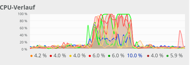
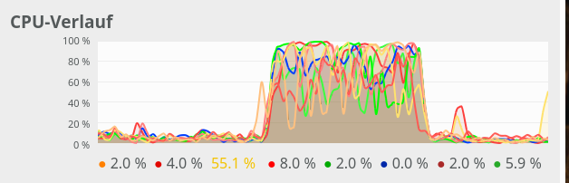
If you raise the number for batches and the number for epochs you will pretty soon realize that writing continuous output to a Jupyter cell costs CPU-time. You will also notice strange things regarding performance, multithreading and the use of the Linalg library OpenBlas on Linux system. I have discussed this extensively in a previous article in this blog:
Linux, OpenBlas and Numpy matrix multiplications – avoid using all processor cores

So, for another tests we set the following environment variable for the shell in which we start our Jupyter notebook:

export OPENBLAS_NUM_THREADS=4

This is appropriate for my Quad-core CPU with hyperthreading. You may choose a different parameter on your system!

We furthermore stop printing in the epoch loop by editing the call to function “_fit()”:

self._fit(b_print=False, b_measure_batch_time=False)

We change our parameter setting to:

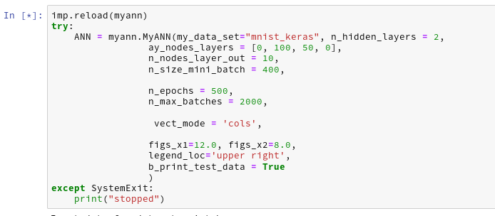
Then the last output lines become:

The node numbers for the 4 layers are : 
[784 100  50  10]

Shape of weight matrix between layers 0 and 1 (100, 785)
Creating weight matrix for layer 1 to layer 2
Shape of weight matrix between layers 1 and 2 = (50, 101)
Creating weight matrix for layer 2 to layer 3
Shape of weight matrix between layers 2 and 3 = (10, 51)

The activation function of the standard neurons was defined as "sigmoid"
The activation function gives for z=2.0:  0.8807970779778823

The output function of the neurons in the output layer was defined as "sigmoid"
The output function gives for z=2.0:  0.8807970779778823
num of mini_batches = 150

number of batches : 150
length of first batch : 400
length of last batch : 400


 ------
Total training Time_CPU:  146.44446582399905

Stopping program regularily
stopped

Good !
The time required to repeat this kind of forward propagation for a network with only one hidden layer with 50 neurons and 1000 epochs is around 160 secs. As backward propagation is not much more complex than forward propagation this already indicates that we should be able to train such a most simple MLP with 60000 28×28 images in less than 10 minutes on a standard CPU.

Conclusion

In this article we saw that coding forward propagation is a pretty straight-forward exercise with Numpy! The tricky thing is to understand the way numpy.dot() handles vectorizing of a matrix product and which structure of the matrices is required to get the expected numbers!

In the next article

A simple program for an ANN to cover the Mnist dataset – IV – the concept of a cost or loss function

we shall start working on cost and gradient calculation.


Linux, OpenBlas and Numpy matrix multiplications – avoid using all processor cores

Recently, I tested the propagation methods of a small Python3/Numpy class for a multilayer perceptron [MLP]. I unexpectedly ran into a performance problem with OpenBlas.

The problem had to do with the required vectorized matrix operations for forward propagation – in my case through an artificial neural network [ANN] with 4 layers. In a first approach I used 784, 100, 50, 10 neurons in 4 consecutive layers of the MLP. The weight matrices had corresponding dimensions.

The performance problem was caused by extensive multi-threading; it showed a strong dependency on mini-batch sizes and on basic matrix dimensions related to the neuron numbers per layer:

  • For the given relatively small number of neurons per layer and for mini-batch sizes above a critical value (N > 255) OpenBlas suddenly occupied all processor cores with a 100% work load. This had a disastrous impact on performance.
  • For neuron numbers as 784, 300, 140, 10 OpenBlas used all processor cores with a 100% work load right from the beginning, i.e. even for small batch sizes. With a seemingly bad performance over all batch sizes – but decreasing somewhat with large batch sizes.

This problem has been discussed elsewhere with respect to the matrix dimensions relevant for the core multiplication and summation operations – i.e. the neuron numbers per layer. However, the vectorizing aspect of matrix multiplications is interesting, too:

One can imagine that splitting the operations for multiple independent test samples is in principle ideal for multi-threading. So, using as many processor cores as possible (in my case 8) does not look like a wrong decision of OpenBlas at first.

Then I noticed that for mini-batch sizes “N” below a certain number (N < 250) the system only seemed to use up to 3-4 cores; so there remained plenty of CPU capacity left for other tasks. Performance for N < 250 was better by at least a factor of 2 compared to a situation with an only slightly bigger batch size (N ≥ 260). I got the impression that OpenBLAS under certain conditions just decides to use as many threads as possible – which no good outcome.

In the last years I sometimes had to work with optimizing multi-threaded database operations on Linux systems. I often got the impression that you have to be careful and leave some CPU resources free for other tasks and to avoid heavy context switching. In addition bottlenecks appeared due to the concurrent access of may processes to the CPU cache. (RAM limitations were an additional factor; but this should not be the case for my Python program.) Furthermore, one should not forget that Python/Numpy experiments on Jupyter notebooks require additional resources to handle the web page output and page update on the browser. And Linux itself also requires some free resources.

So, I wanted to find out whether reducing the number of threads – or available cores – for Numpy and OpenBlas would be helpful in the sense of an overall gain in performance.

All data shown below were gathered on a desktop system with some background activity due to several open browsers, clementine and pulse-audio as active audio components, an open mail client (kontact), an open LXC container, open Eclipse with Pydev and open ssh connections. Program tests were performed with the help of Jupyter notebooks. Typical background CPU consumption looks like this on Ksysguard:

Most of the consumption is due to audio. Small spikes on one CPU core due to the investigation of incoming mails were possible – but always below 20%.

Basics

One of
the core ingredients to get an ANN running are matrix operations. More precisely: multiplications of 2-dim Numpy matrices (weight matrices) with input vectors. The dimensions of the weight matrices reflect the node-numbers of consecutive ANN-layers. The dimension of the input vector depends on the node number of the lower of two neighbor layers.

However, we perform such matrix operations NOT sequentially sample for sample of a collection of training data – we do it vectorized for so called mini-batches consisting of between 50 and 600000 individual samples of training data. Instead of operating with a matrix on just one feature vector of one training sample we use matrix multiplications whereby the second matrix often comprises many vectors of data samples.

I have described such multiplications already in a previous blog article; see Numpy matrix multiplication for layers of simple feed forward ANNs.

In the most simple case of an MLP with e.g.

  • an input layer of 784 nodes (suitable for the MNIST dataset),
  • one hidden layer with 100 nodes,
  • another hidden layer with 50 nodes
  • and an output layer of 10 nodes (fitting again the MNIST dataset)

and “mini”-batches of different sizes (between 20 and 20000). An input vector to the first hidden layer has a dimension of 100, so the weight matrix creating this input vector from the “output” of the MLP’s input layer has a shape of 784×100. Multiplication and summation in this case is done over the dimension covering 784 features. When we work with mini-batches we want to do these operations in parallel for as many elements of a mini-batch as possible.

All in all we have to perform 3 matrix operations

(784×100) matrix on (784)-vector, (100×50) matrix on (100)-vector, (50×10) matrix on (50) vector

on our example ANN with 4 layers. However, we collect the data for N mini-batch samples in an array. This leads to Numpy matrix multiplications of the kind

(784×100) matrix on an (784, N)-array, (100×50) matrix on an (100, N)-array, (50×10) matrix on an (50, N)-array.

Thus, we deal with matrix multiplications of two 2-dim matrices. Linear algebra libraries should optimize such operations for different kinds of processors.

The reaction of OpenBlas to an MLP with 4 layers comprising 784, 100, 50, 10 nodes

On my Linux system Python/Numpy use the openblas-library. This is confirmed by the output of command “np.__config__.show()”:

openblas_info:
    libraries = ['openblas', 'openblas']
    library_dirs = ['/usr/local/lib']
    language = c
    define_macros = [('HAVE_CBLAS', None)]
blas_opt_info:
    libraries = ['openblas', 'openblas']
    library_dirs = ['/usr/local/lib']
    language = c
    define_macros = [('HAVE_CBLAS', None)]
openblas_lapack_info:
    libraries = ['openblas', 'openblas']
    library_dirs = ['/usr/local/lib']
    language = c
    define_macros = [('HAVE_CBLAS', None)]
lapack_opt_info:
    libraries = ['openblas', 'openblas']
    library_dirs = ['/usr/local/lib']
    language = c
    define_macros = [('HAVE_CBLAS', None)]

and by

(ml1) myself@mytux:/projekte/GIT/ai/ml1/lib64/python3.6/site-packages/numpy/core> ldd  _multiarray_umath.cpython-36m-x86_64-linux-gnu.so
        linux-vdso.so.1 (0x00007ffe8bddf000)
        libopenblasp-r0-2ecf47d5.3.7.dev.so => /projekte/GIT/ai/ml1/lib/python3.6/site-packages/numpy/core/./../.libs/libopenblasp-r0-2ecf47d5.3.7.dev.so (0x00007fdd9d15f000)
        libm.so.6 => /lib64/libm.so.6 (0x00007fdd9ce27000)
        libpthread.so.0 => /lib64/libpthread.so.0 (0x00007fdd9cc09000)
        libc.so.6 => /lib64/libc.so.6 (0x00007fdd9c84f000)
        /lib64/ld-
linux-x86-64.so.2 (0x00007fdd9f4e8000)
        libgfortran-ed201abd.so.3.0.0 => /projekte/GIT/ai/ml1/lib/python3.6/site-packages/numpy/core/./../.libs/libgfortran-ed201abd.so.3.0.0 (0x00007fdd9c555000)

In all tests discussed below I performed a series of calculations for different batch sizes

N = 50, 100, 200, 250, 260, 500, 2000, 10000, 20000

and repeated the full forward propagation 30 times (corresponding to 30 epochs in a full training series – but here without cost calculation and weight adjustment. I just did forward propagation.)

In a first experiment, I did not artificially limit the number of cores to be used. Measured response times in seconds are indicated in the following plot:

Runtime for a free number of cores to use and different batch-sizes N

We see that something dramatic happens between a batch size of 250 and 260. Below you see the plots for CPU core consumption for N=50, N=200, N=250, N=260 and N=2000.

N=50:

N=200:

N=250:

N=260:

N=2000:

The plots indicate that everything goes well up to N=250. Up to this point around 4 cores are used – leaving 4 cores relatively free. After N=260 OpenBlas decides to use all 8 cores with a load of 100% – and performance suffers by more than a factor of 2.

This result support the idea to look for an optimum of the number of cores “C” to use.

The reaction of OpenBlas to an MLP with layers comprising 784, 300, 140, 10 nodes

For a MLP with neuron numbers (784, 300, 140, 10) I got the red curve for response time in the plot below. The second curve shows what performance is possible with just using 4 cores:

Note the significantly higher response times. We also see again that something strange happens at the change of the batch-size from 250 to 260.

The 100% CPU
consumption even for a batch-size of only 50 is shown below:

Though different from the first test case also these plots indicate that – somewhat paradoxically – reducing the number of CPU cores available to OpenBlas could have a performance enhancing effect.

Limiting the number of available cores to OpenBlas

A bit of Internet research shows that one can limit the number of cores to use by OpenBlas e.g. via an environment variable for the shell, in which we start a Jupyter notebook. The relevant command to limit the number of cores “C” to 3 is :

export OPENBLAS_NUM_THREADS=3

Below you find plots for the response times required for the batch sizes N listed above and core numbers of

C=1, C=2, C=3, C=4, C=5, C=6, C=7, C=8 :

For C=5 I did 2 different runs; the different results for C=5 show that the system reacts rather sensitively. It changes its behavior for larger core number drastically.

We also find an overall minimum of the response time:
The overall optimum occurs for 400 < N < 500 for C=1, 2, 3, 4 – with the minimum region being broadest for C=3. The absolute minimum is reached on my CPU for C=4.

We understand from the plots above that the number of cores to use become hyper-parameters for the tuning of the performance of ANNs – at least as long as a standard multicore-CPU is used.

CPU-consumption

CPU consumption for N=50 and C=2 looks like:

For comparison see the CPU consumption for N=20000 and C=4:

CPU consumption for N=20000 and C=6:

We see that between C=5 and C=6 CPU resources get heavily consumed; there are almost no reserves left in the Linux system for C ≥ 6.

Dependency on the size of the weight-matrices and the node numbers

For a full view on the situation I also looked at the response time variation with node numbers for a given number of CPU cores.

For C=4 and node number cases

  • 784, 300, 140, 10
  • 784, 200, 100, 10
  • 784, 100, 50, 10
  • 784, 50, 20, 10

I got the following results:

There is some broad variation with the weight-matrix size; the bigger the weight-matrix the longer the calculation time. This is, of course, to be expected. Note that the variation with the batch-size number is relatively smooth – with an optimum around 400.

Now, look at the same plot for C=6:

Note that the response time is significantly bigger in all cases compared to the previous situation with C=4. In cases of a large matrix by around 36% for N=2000. Also the variation with batch-size is more pronounced.

Still, even with 6 cores you do not get factors between 1.4 and 2.0 as compared to the case of C=8 (see above)!

Conclusion

As I do not know what the authors of OpenBlas are doing exactly, I refrain from technically understanding and interpreting the causes of the data shown above.

However, some consequences seem to be clear:

  • It is a bad idea to provide all CPU cores to OpenBlas – which unfortunately is the default.
  • The data above indicate that using only 4 out of 8 core threads is reasonable to get an optimum performance for vectorized matrix multiplications on my CPU.
  • Not leaving at least 2 CPU cores free for other tasks is punished by significant performance losses.
  • When leaving the decision of how many cores to use to OpenBlas a critical batch-size may exist for which the performance suddenly breaks down due to heavy multi-threading.

Whenever you deal with ANN or MLP simulations on a standard CPU (not GPU!) you should absolutely care about how many cores and related threads you want to offer to OpenBlas. As far as I understood from some Internet articles the number of cores to be used can be not only be controlled by Linux (shell) environment variables but also by os-commands in a Python program. You should perform tests to find optimum values for your CPU.

Links

stackoverflow: numpy-suddenly-uses-all-cpus

stackoverflow: run-openblas-on-multicore

stackoverflow: multiprocessing-pool-makes-numpy-matrix-multiplication-slower

scicomp: why-isnt-my-matrix-vector-multiplication-scaling/1729

Setting the number of threads via Python
stackoverflow:
set-max-number-of-threads-at-runtime-on-numpy-openblas

codereview.stackexchange: better-way-to-set-number-of-threads-used-by-numpy


Eclipse, PyDev, virtualenv and graphical output of matplotlib on KDE – I

When you enter the field of machine learning [ML] and Artificial Intelligence [AI] there is no way around Python. And whilst studying books like “A. Geron’s Machine Learning with SciKit-Learn & TensorFlow” [1] or F. Chollet’s “Deep learning with Python and Keras” [2] one understands quickly: You do not learn by reading, but by doing experiments.

For me this meant to both improve my basic Python knowledge and to set up a reasonable working environment on my Linux workstation (with Opensuse Leap Linux and KDE). The named books recommend using “Jupyter notebooks” – and I must say, Jupyter environments are fun to use. However, as soon as I started with more complex program variations I began missing an IDE. I think that in the end Python code must be organized in a more systematic way than during experiments with Jupyter notebooks. A Jupyter notebook serves one purpose, a Python IDE a supplemental one.

A natural choice for an IDE based on opensource tools is Eclipse with PyDev. After a basic setup I stumbled across two problems:

  • For projects a so called “virtual” Python environment is useful, which encapsulates a defined mix of Python and library versions. How to use “virtualenv” within PyDev and its Python specific console?
  • Quite often the results of ML/AI-experiments need to be represented in a graphical way. Browser based “Jupyter notebooks” make the use of graphics easy by using browser capabilities. But how to use Python’s matplotlib in my Opensuse/KDE/Eclipse environment?

In this article I address the steps to setup Eclipse/PyDev in such a way that both points are covered. I do this for an Opensuse Leap system, but a transfer to other Linux distributions should be simple. The group of readers I address is either ML-interested folks for whom Eclipse is a new environment or people as me who know Eclipse but not the PyDev plugin. People who already work with PyDev will probably not learn anything new.

Step 1: Install Eclipse

A basic Eclipse installation is a straightforward business on most Linux distributions ( see e.g.: https://simopr.wordpress.com/2016/05/26/install-eclipse-ide-on-opensuse-leap-42/). I will, therefore, not cover this topic in detail here. You first need to install a Java Runtime environment (on Opensuse via the RPM java-10-openjdk), if not yet provided by your distribution. A current version of Eclipse can be downloaded from the site
https://www.eclipse.org/downloads/packages/.
(Actually, I used my already installed Eclipse photon version 4.9.0 of September 2018 – which works pretty well for me. But the present 2019 RC3 candidate of Eclipse should work as well.)

To my knowledge there is no special Eclipse package for Python developers; as a PHP-developer I choose the package for PHP-developers for a basic Eclipse installation and install the required Python PyDev packages afterwards.

You download your chosen tar.gz-file from the Eclipse site named above, save it and then expand its contents into a suitable directory of your Linux system (in my case into “/projects/eclipse”). Then you can directly start the executable “eclipse”-file there – e.g. in a terminal.

Then you need to define your path for a “workspace” for your Python projects. Note that the workspace is not necessarily identical with a root directory for all your project files; a workspace instead gathers information on your configuration settings for Eclipse and defined projects. The project files themselves, however, can be located in a very different place – e.g. in a directory defined for your local GIT platform – in my case below “/projects/GIT/…”.

Eventually, you get a full fledged Eclipse IDE interface, which you
can customize (see “Window >> “Preferences”). This is beyond the scope of this article; I give however some hints regarding color. You can e.g. customize editor and console colors for specific programming languages within Eclipse.

However, regarding certain application control elements you may nevertheless run into trouble regarding the definition of colors; one reason is that on a Qt5-based KDE desktop the end result may depend both on Eclipse settings and also on desktop design schemes for GTK2/GTK3 applications as Eclipse. This type of dependency requires experiments. So, what exactly do I use?

Within Eclipse itself I use the “Dark Theme” – to avoid an eye sore whilst programming.

Regarding my KDE desktop I use a standard Breeze Desktop Scheme with Elegance-Design and the Standard Color Theme (with the activation flag for non-Qt-applications set). KDE application design elements, however, are taken from the Adwaita-Scheme. For GTK2 applications on KDE I prefer the Clearlooks-design, for GTK3 applications – as Eclipse (> 4.9.0) – again Adwaita. This combination gives me a sufficient foreground/background-contrast for control elements like checkboxes, radio buttons, …

A last convenience point: In a graphical desktop environment as KDE you will of course add some icon to your desktop (in my case with a reference to the file “projects/eclipse/eclipse”) to reduce the starting process to a click.

Step 2: Basic Python packages on the system level

I assume that you have already installed Python in your Linux-(Opensuse)-system. In my environment I use the Python 3.6 RPM-packages from the standard repositories for Opensuse Leap 15.0:
https://download.opensuse.org/distribution/ leap/15.0/repo/oss/
https://download.opensuse.org/update/ leap/15.0/oss/.

The number of available Python library packages is quite big; what libraries you should install depends on your programming objectives. You need at least the basic “python3” package. Another “must”, in my opinion, is the package “python3-pip“; it enables us to perform specific package installations for our “virtual Python environment” later on.

As a basic ingredient for graphics you may also install suitable libraries for your Linux desktop environment. In my case this is KDE – so I installed the packages “python3-qt5″, python-qt5-utils” and also “python3-qt5-devel” to be on the safe side. However, as we shall see we may need Qt5-packages within a project environment, too. That is where Python’s internal “pip” mechanism enters the game.

Below we shall perform the installation of the “virtualenv” package to demonstarte the usage of “pip” or “pip3” in a Python3-environment. As a first step I provide myself (i.e. user “myself”) with a current version of “pip3”:

myself@mytux:~> pip3 --version
pip 19.1.0 from /home/myself/.local/lib/python3.6/site-packages/pip (python 3.6)
myself@mytux:~> pip3 install --user --
upgrade pip
Collecting pip
  Downloading https://files.pythonhosted.org/packages/5c/e0/be401c003291b56efc55aeba6a80ab790d3d4cece2778288d65323009420/pip-19.1.1-py2.py3-none-any.whl (1.4MB)
     |████████████████████████████████| 1.4MB 1.0MB/s 
Installing collected packages: pip
  Found existing installation: pip 19.1                                                                                                                                                 
    Uninstalling pip-19.1:                                                                                                                                                              
      Successfully uninstalled pip-19.1                                                                                                                                                 
Successfully installed pip-19.1.1                                                                                                                                                       
myself@mytux:~> pip3 --version
pip 19.1.1 from /home/myself/.local/lib/python3.6/site-packages/pip (python 3.6)

You see that the parameter “–user” already lead to a personal configuration of basic Python packages (within my home-directory). But we shall specify a project specific environment in the fourth step.

Step3: Working directory for our ML-project

We now define a base directory “ai” for future experiments.

myself@mytux:~> export AI_PATH ="/projekte/GIT/ai/"
myself@mytux:~> mkdir -p $AI_PATH

A sub-directory “ml1” shall provide the environment for a bunch of initial basic ML-experiments and related Python code files, libraries, Jupyter notebooks, etc.. We create this “ml1” directory as a base for a “virtual” Python environment.

Step 4: Prepare a virtual Python environment via virtualenv and working directories

Python installations allow for the definition of a so called “virtual environment” for projects via the “virtualenv” add-on. Among other things “virtualenv” lets you define a project specific configuration with Python and library versions in a consistent reproducible state. This in turn gives you a base for the “configuration management” of complex endeavors; therefore, I strongly recommend to make use of this feature – also in combination with PyDev: .

myself@mytux:~> pip3 install --user --upgrade virtualenv
Collecting virtualenv
  Downloading https://files.pythonhosted.org/packages/ca/ee/8375c01412abe6ff462ec80970e6bb1c4308724d4366d7519627c98691ab/virtualenv-16.6.0-py2.py3-none-any.whl (2.0MB)
     |████████████████████████████████| 2.0MB 1.6MB/s 
Installing collected packages: virtualenv
  Found existing installation: virtualenv 16.5.0
    Uninstalling virtualenv-16.5.0:
      Successfully uninstalled virtualenv-16.5.0
Successfully installed virtualenv-16.6.0
myself@mytux:~> virtualenv --version
16.6.0
myself@mytux:~>

Now we can use “virtualenv” to setup the virtual Python environment for “ml1” in our “ai”-directory:

myself@mytux:~> cd /projekte/GIT/ai/
myself@mytux:/projekte/GIT/ai> virtualenv ml1
Using base prefix '/usr'
  No LICENSE.txt / LICENSE found in source
New python executable in /projekte/GIT/ai/ml1/bin/python3
Also creating executable in /projekte/GIT/ai/ml1/bin/python
Installing setuptools, pip, wheel...
done.
myself@mytux:/projekte/GIT/ai> la ml1
insgesamt 20
drwxr-xr-x 5 myself users 4096 25. Mai 15:05 .
drwxr-xr-x 3 myself users 4096 25. Mai 15:05 ..
drwxr-xr-x 2 myself users 4096 25. Mai 15:05 bin
drwxr-xr-x 2 myself users 4096 25. Mai 15:05 include
drwxr-xr-x 3 myself users 4096 25. Mai 15:05 lib
lrwxrwxrwx 1 myself users    3 25. Mai 15:05 lib64 -> lib
myself@mytux:/projekte/GIT/ai> la ml1/bin
insgesamt 72
drwxr-xr-x 2 myself users  4096 25. Mai 15:05 .
ndrwxr-xr-x 5 myself users  4096 25. Mai 15:05 ..
-rw-r--r-- 1 myself users  2096 25. Mai 15:05 activate
-rw-r--r-- 1 myself users  1428 25. Mai 15:05 activate.csh
-rw-r--r-- 1 myself users  3052 25. Mai 15:05 activate.fish
-rw-r--r-- 1 myself users  1804 25. Mai 15:05 activate.ps1
-rw-r--r-- 1 myself users  1512 25. Mai 15:05 activate_this.py
-rw-r--r-- 1 myself users  1150 25. Mai 15:05 activate.xsh
-rwxr-xr-x 1 myself users   249 25. Mai 15:05 easy_install
-rwxr-xr-x 1 myself users   249 25. Mai 15:05 easy_install-3.6
-rwxr-xr-x 1 myself users   231 25. Mai 15:05 pip
-rwxr-xr-x 1 myself users   231 25. Mai 15:05 pip3
-rwxr-xr-x 1 myself users   231 25. Mai 15:05 pip3.6
lrwxrwxrwx 1 myself users     7 25. Mai 15:05 python -> python3
-rwxr-xr-x 1 myself users 10456 25. Mai 15:05 python3
lrwxrwxrwx 1 myself users     7 25. Mai 15:05 python3.6 -> python3
-rwxr-xr-x 1 myself users  2338 25. Mai 15:05 python-config
-rwxr-xr-x 1 myself users   227 25. Mai 15:05 wheel
myself@mytux:/projekte/GIT/ai> 

You see that a whole directory structure was established – with Python3 executables copied from our basic system installation. We can fully use this Python environment already on the command line (of a terminal window). However, we need to activate it so that its files and libs are really used:

myself@mytux:/projekte/GIT/ai/ml1> source bin/activate  
(ml1) myself@mytux:/projekte/GIT/ai/ml1> python3 
Python 3.6.5 (default, Mar 31 2018, 19:45:04) [GCC] on linux
Type "help", "copyright", "credits" or "license" for more information.
>>> print("Hello World!")
Hello World!
>>> quit()
(ml1) myself@mytux:/projekte/GIT/ai/ml1> pip3 install --upgrade jupyter                                                                                                                      
Collecting jupyter                                                                                                                                                                      
  Using cached https://files.pythonhosted.org/packages/83/df/0f5dd132200728a86190397e1ea87cd76244e42d39ec5e88efd25b2abd7e/jupyter-1.0.0-py2.py3-none-any.whl                            
Collecting notebook (from jupyter)
...
..Successfully built pyrsistent
Installing collected packages: Send2Trash, ipython-genutils, decorator, six, traitlets, jupyter-core, MarkupSafe, jinja2, pyzmq, python-dateutil, tornado, jupyter-client, backcall, pickleshare, wcwidth, prompt-toolkit, ptyprocess, pexpect, pygments, parso, jedi, ipython, ipykernel, prometheus-client, pyrsistent, attrs, jsonschema, nbformat, terminado, entrypoints, mistune, webencodings, bleach, testpath, defusedxml, pandocfilters, nbconvert, notebook, jupyter-console, widgetsnbextension, ipywidgets, qtconsole, jupyter
Successfully installed MarkupSafe-1.1.1 Send2Trash-1.5.0 attrs-19.1.0 backcall-0.1.0 bleach-3.1.0 decorator-4.4.0 defusedxml-0.6.0 entrypoints-0.3 ipykernel-5.1.1 ipython-7.5.0 ipython-genutils-0.2.0 ipywidgets-7.4.2 jedi-0.13.3 jinja2-2.10.1 jsonschema-3.0.1 jupyter-1.0.0 jupyter-client-5.2.4 jupyter-console-6.0.0 jupyter-core-4.4.0 mistune-0.8.4 nbconvert-5.5.0 nbformat-4.4.0 notebook-5.7.8 pandocfilters-1.4.2 parso-0.4.0 pexpect-4.7.0 pickleshare-0.7.5 prometheus-client-0.6.0 prompt-toolkit-2.0.9 ptyprocess-0.6.0 pygments-2.4.1 pyrsistent-0.15.2 python-dateutil-2.8.0 pyzmq-18.0.1 qtconsole-4.5.0 six-1.12.0 terminado-0.8.2 testpath-0.4.2 tornado-6.0.2 traitlets-4.3.2 wcwidth-0.1.7 webencodings-0.5.1 widgetsnbextension-3.4.2
(ml1) myself@mytux:/projekte/GIT/ai/ml1/include> cd ../bin
(ml1) myself@mytux:/projekte/GIT/ai/ml1/bin> la
insgesamt 152
drwxr-xr-x 2 myself users  4096 26. Mai 14:22 .
drwxr-xr-x 7 myself users  4096 26. Mai 14:22 ..
-rw-r--r-- 1 myself users  2096 25. Mai 15:05 activate
-rw-r--r-- 1 myself users  1428 25. Mai 15:05 activate.csh
-rw-r--r-- 1 myself users  3052 25. Mai 15:05 activate.fish
n-rw-r--r-- 1 myself users  1804 25. Mai 15:05 activate.ps1
-rw-r--r-- 1 myself users  1512 25. Mai 15:05 activate_this.py
-rw-r--r-- 1 myself users  1150 25. Mai 15:05 activate.xsh
-rwxr-xr-x 1 myself users   249 25. Mai 15:05 easy_install
-rwxr-xr-x 1 myself users   249 25. Mai 15:05 easy_install-3.6
-rwxr-xr-x 1 myself users   250 26. Mai 14:22 iptest
-rwxr-xr-x 1 myself users   250 26. Mai 14:22 iptest3
-rwxr-xr-x 1 myself users   243 26. Mai 14:22 ipython
-rwxr-xr-x 1 myself users   243 26. Mai 14:22 ipython3
-rwxr-xr-x 1 myself users   232 26. Mai 14:22 jsonschema
-rwxr-xr-x 1 myself users   238 26. Mai 14:22 jupyter
-rwxr-xr-x 1 myself users   252 26. Mai 14:22 jupyter-bundlerextension
-rwxr-xr-x 1 myself users   237 26. Mai 14:22 jupyter-console
-rwxr-xr-x 1 myself users   242 26. Mai 14:22 jupyter-kernel
-rwxr-xr-x 1 myself users   280 26. Mai 14:22 jupyter-kernelspec
-rwxr-xr-x 1 myself users   238 26. Mai 14:22 jupyter-migrate
-rwxr-xr-x 1 myself users   240 26. Mai 14:22 jupyter-nbconvert
-rwxr-xr-x 1 myself users   239 26. Mai 14:22 jupyter-nbextension
-rwxr-xr-x 1 myself users   238 26. Mai 14:22 jupyter-notebook
-rwxr-xr-x 1 myself users   240 26. Mai 14:22 jupyter-qtconsole
-rwxr-xr-x 1 myself users   259 26. Mai 14:22 jupyter-run
-rwxr-xr-x 1 myself users   243 26. Mai 14:22 jupyter-serverextension
-rwxr-xr-x 1 myself users   243 26. Mai 14:22 jupyter-troubleshoot
-rwxr-xr-x 1 myself users   271 26. Mai 14:22 jupyter-trust
-rwxr-xr-x 1 myself users   231 25. Mai 15:05 pip
-rwxr-xr-x 1 myself users   231 25. Mai 15:05 pip3
-rwxr-xr-x 1 myself users   231 25. Mai 15:05 pip3.6
-rwxr-xr-x 1 myself users   234 26. Mai 14:22 pygmentize
lrwxrwxrwx 1 myself users     7 25. Mai 15:05 python -> python3
-rwxr-xr-x 1 myself users 10456 25. Mai 15:05 python3
lrwxrwxrwx 1 myself users     7 25. Mai 15:05 python3.6 -> python3
-rwxr-xr-x 1 myself users  2338 25. Mai 15:05 python-config
-rwxr-xr-x 1 myself users   227 25. Mai 15:05 wheel

Looking into the lib-directory is also informative. I leave this to the user.

(ml1) myself@mytux:/projekte/GIT/ai/ml1/bin> cd ../lib/python3.6/site-package
(ml1) myself@mytux:/projekte/GIT/ai/ml1/lib/python3.6/site-packages> la

Step 5: Install some important libraries for ML studies

As we are occupied with installing packages, let us get some more packages typically required to do experiments for AI/ML:

(ml1) myself@mytux:/projekte/GIT/ai/ml1> pip3 install --upgrade matplotlib numpy pandas scipy scikit-learn
....

Step 6: Install PyDev for Eclipse

The previous steps were all on the level of the Linux-system and/or for a special Python environment for me as a user. But Eclipse does not know anything about Python, yet. We need a special Python environment within Eclipse with suitable editors, project and test environments, configuration options and so on for our Python based machine learning projects.

You find the necessary PyDev plugins for Eclipse at the site http://pydev.sf.net/updates/.

The easiest way to install PyDev is: Add this site to the update configuration of Eclipse – via the menu point “Help >> Install new software”. Click the “Add”-Button there. In the popup you provide a name for the site and its URL. Then you choose this site “to work with” and click on the relevant plugin “PyDev for Eclipse”. If you are a fan of Mylyn you also load the respective package.

Step 7: Change to a PyDev perspective within Eclipse

After having installed the PyDev packages we can start Eclipse and change
the layout by choosing a Python specific “perspective“.

We start with the menu point
“Window >> Perspective >> Open Perspective >> Other …”

Then we choose “PyDev” and end up with the a layout of Eclipse similar to the following (you may have some other position arrangements of the sub-windows):

On the left side you see some projects, which I had set up already. (As I integrate some of my Python experiments with PHP-programs the reader may detect some PHP-projects, too …). In the lower right part of the IDE we see a console view for interactive python commands. I come back to this point below.

Step 8: Add a Python project in Eclipse for our virtual environment ml1

We now create a new project which shall be related to our directory “/projekte/GIT/ai/ml1”. A right mouse click into the leftmost area gives us:

On the next popup we choose a “PyDev”-project type.

On the third screen we first enter our path “/projekte/GIT/ai/ml1” – with this setting we see all the modules and libraries loaded for our virtual environment in Eclipse, too.

The important interpreter setting – it decides on the usage of our virtualenv
Really interesting is the field for the choice of an “Interpreter“. Here we get the option to refer to our “virtual environment”. When we click on the blue link we can configure an interpreter and related path settings. On the opening popup window we enter the path to the interpreter of our ml1-environment, i.e. to “/projekte/GIT/ai/ml1/bin/python3.6“.

We go on and get

Important: We do not delete the references to the systems libraries here!

We move on and come back to our project definition window – we now
choose the interpreter “python_ml1” which we defined a minute ago.

On the next screen we do not yet have any other projects to be referenced.

So we finish and get our first Python3 project:

Enough for today. In the second article

Eclipse, PyDev, virtualenv and graphical output of matplotlib on KDE – II

of this series we shall use a Python-console within Eclipse for interactive coding and the display of results. We shall see that we need additional settings to get matplotlib to work.

Stay tuned …

Links

https://www.caktusgroup.com/blog/2011/08/31/getting-started-using-python-eclipse/