
I continue my series of articles on a CNN for the MNIST dataset.
A simple CNN for the MNIST dataset – IX – filter visualization at a convolutional layer
A simple CNN for the MNIST dataset – VIII – filters and features – Python code to visualize patterns which activate a map strongly
A simple CNN for the MNIST dataset – VII – outline of steps to visualize image patterns which trigger filter maps
A simple CNN for the MNIST dataset – VI – classification by activation patterns and the role of the CNN’s MLP part
A simple CNN for the MNIST dataset – V – about the difference of activation patterns and features
A simple CNN for the MNIST dataset – IV – Visualizing the activation output of convolutional layers and maps
A simple CNN for the MNIST dataset – III – inclusion of a learning-rate scheduler, momentum and a L2-regularizer
A simple CNN for the MNIST datasets – II – building the CNN with Keras and a first test
A simple CNN for the MNIST datasets – I – CNN basics
In the last article we harvested the fruits of previous efforts. We produced a variety of input image patterns which triggered certain maps of the innermost convolutional layer of our CNN and the filters behind it maximally. I called such pixel-patterns OIPs. (I am still careful to avoid the expression “feature”, which is used by many authors as a term describing a physical entity identified by the human brain. A connotation which I do not like …)
Although my code for creating OIPs allows for a variation of fluctuations on 4 different length scales it proved to be hard to find OIPs for quite a lot of maps at the highest convolutional layer and for their filters. I could not always find a combination of initial random pixel fluctuations which led to loss values > 0. More precisely: I did not find a pattern by trial and error on a reasonable short timescale of some minutes.
We already know that OIP pixel patterns for the innermost convolutional layer are a bit artificial:
- They are idealizations; the displayed pattern may not be present in the same form in the real input images which were used during training.
- They may contain repetitions of sub-patterns at different positions.
The images in the last articles showed us in addition that some maps at the innermost Conv-layer are sensitive to rather complicated and specific patterns on relatively large length scales.
This is to be expected as at least filters on the higher convolutional levels accumulate information on a coarse level of image coverage: Filtered information coming from original large areas of the image are in the end convoluted down to grids of (3×3) neurons, i.e. onto low resolution maps. Filters at this convolutional depth can therefore require relatively large scale patterns to be passed. So, it is no real wonder that some maps do not react at all to random statistical fluctuations on very short length scales, e.g. on a two pixel scale. The activation of the respective neurons may stay at zero.
In this article I shall describe a simple method which allowed me to create OIP patterns for around half of the maps (at the 3d Conv-level) for which I did not have any luck before. This is done by a “precursor run” which tests the reaction of a map to a large sample of input images with pattern variations on relatively long length scales.
Systematic analysis? My simple approach …
What is the basic idea? Let us assume that we cover the original image surface by a a grid of squares, e.g. by 16 (7×7)-squares – where (7×7) means a square with a side length of 7 pixels. We then assign a constant grey-value to all the pixels in such a square. Instead of picking random values in the range [0, 255] we use a limited number of N distinct normalized values in an interval [0, 1].
We then investigate all combinations of distinct value distributions across the 16 squares. For each combination we construct an input image with bicubic interpolation on the original (28×28) scale and standardize the resulting distribution of pixel values. (The standardization is required for my CNN, which was trained on standardized images). Thus we produce a (huge) number of input images with smooth large scale fluctuations, which we then can present to our OIP-optimization algorithm for a test of a map’s reaction.
Do we have a chance to find OIPs by systematic trials?
Now, do we have a real chance to work a bit more systematically with the described approach? Unfortunately, the answer is: Not really, at least not with a PC equipment and for fluctuations at middle length scales with more than 5 distinct pixel values. The reason in terms of Fourier series’ is that the number of amplitude combinations for multiple sinus waves grows exponentially with a defined number of discrete amplitudes values out of an interval.
We see the limitations already in our simplified approach. Let us assume that we pick 5 distinct and normalized pixel values in the interval ]0, 1[. Let us further assume that we cover the whole image area (of a size 28×28) with a grid of (9×9) squares, each with a constant pixel value. (We ignore the fact that 28/9 = 3.11 and trust in bicubic interpolation to take care of the 0.11 🙂 )
Even under these conditions we get already around 5**9 = 1.953 million pattern variations for which we have to test a map’s response. For each of these patterns we would have to follow at least 4 to 10 iterations (= epochs) of the optimization loop to identify the input image as a promising candidate for a full optimization or not. This means that we need 8 to 20 million full gradient calculations on a parameter space with 784 (=28×28) dimensions. Hard work even for graphic cards (at the consumer level). At smaller length scales, as induced e.g. by a (7×7) coverage grid, we go far beyond standard calculation capacities on PC hardware.
What was/is within my computational reach? If we reduced the number of distinct pixel values to 3 (e.g.: 0.2, 0.5, 0.8) and concentrated on large scale fluctuations – e.g. based on (9×9) squares – we would have around 19700 combinations to investigate.
I had to work a bit on the respective Python code to get it run under Tensorflow 2.2.1/Cuda 10.2 with a reasonable percentage of around 30% on a graphics card. With 10 epochs for an optimization trial run for each image a complete run over 20000 images takes less than 5 minutes on my old GTX960 graphics card. With a modern card, a recent CPU and some more optimization one would probably arrive at values significantly below a minute. So, systematically working with large scale fluctuations is possible on PC-equipment!
Note that a coverage of the image surface with (9×9)-squares corresponds to the resolution which the (3×3)-maps of the innermost Conv-layers represent! (Including padding in the filter definitions). I assume that it is reasonable to work and test on this scale.
Selection of 8 promising candidates out of 19683
So, I added some “precursor” methods to my class My_OIP to prepare and perform systematic runs for all of the maps for which I had not found a pattern, yet. I chose the following 3 discrete pixel values: [0.2, 0.5, 0.8].
The resulting (9×9) images where rescaled with a bicubic interpolation to the MNIST size of (28×28) and afterwards standardized.
During the test of a map’s response I selected 8 candidates out of 19683 for subsequent thorough optimization runs with 1200 epochs. The selection was done by looking at the largest loss values reached after 10 optimization epochs. I then applied the procedure to all 67 maps for which I had not got an OIP, yet.
Note that we cannot be sure whether 10 optimization iterations really give us a perfect indication of the highest loss values which would be reached after a full optimization run with 600 to 1200 epochs. So, it is worthwhile to play around with the number of test epochs; the selection of the input fluctuation patterns may change.
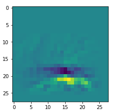
I got results then for 33 of the maps which had no OIP. I present the OIP-images below. The results cover almost 50% of the missing OIPs. So, my computational efforts were well invested.
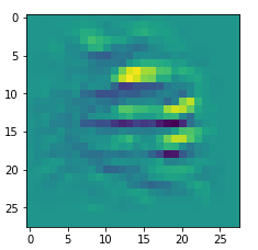
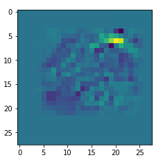
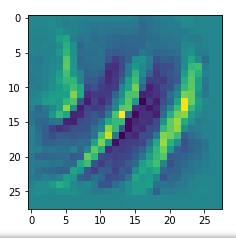
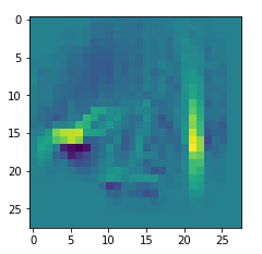
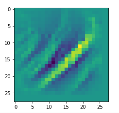
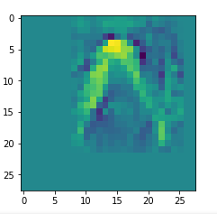
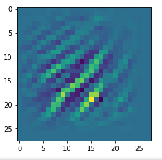
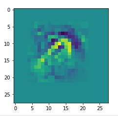
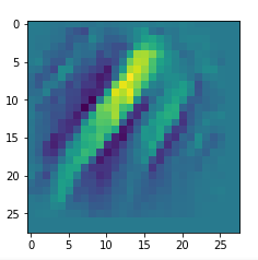
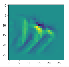
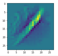
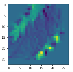
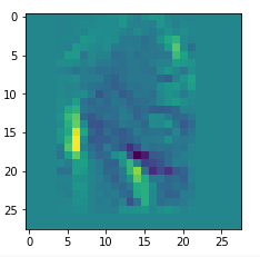
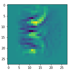
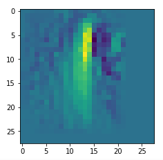
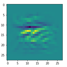
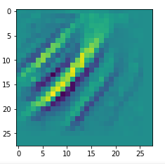
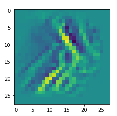
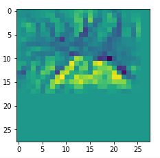
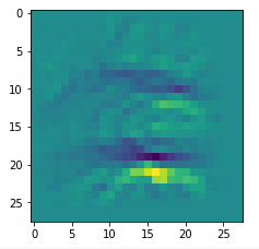
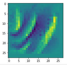
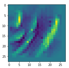
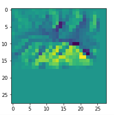
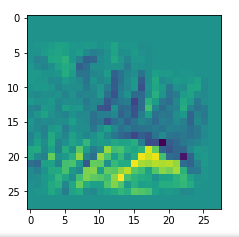
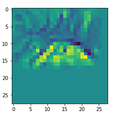
OIPs for additional 33 maps
Below I present MNIST-related OIP-images for the maps with the following indices on the 3rd Conv-layer of my (!) CNN ):
1, 3, 9, 15, 16, 29, 35, 37, 38, 44, 46, 50, 51, 55, 59, 60, 70, 78, 81, 91, 93, 94, 96, 97, 101, 104, 108, 109, 111, 112, 116, 122, 125.
This time without contrast enhancement – as I was too lazy to integrate it into the precursor code.


CNNs are fun, aren’t they?
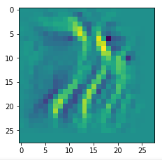
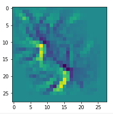
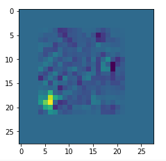
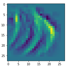
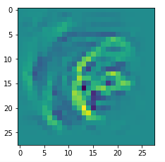
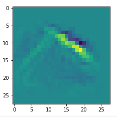
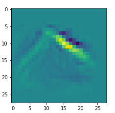
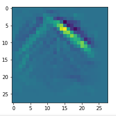
Unique OIPs?
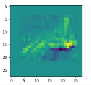
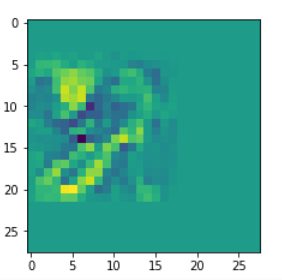
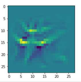
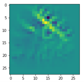
An interesting question is: Are the OIPs really unique per map in the sense that we produce the same OIP-images for different fluctuations on the input images? Well, there is some unique overall form of the patterns, but there may occur translations in position and there may be differences in details. Below, I show you different derived images for some maps:
Map 46:

Map 81:
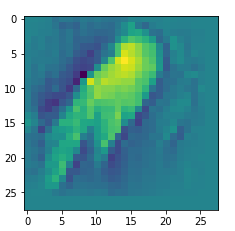

Map 116:
Map 125:
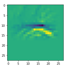
Map 127:
Conclusion
By a systematic investigation of the reaction of maps to large scale fluctuations we can find OIPs for maps where a trial and error approach is not sufficient to trigger a response of the filters. I will discuss the Python code for a related “precursor run” in my next post
A simple CNN for the MNIST dataset – XI – Python code for filter visualization and OIP detection.