
In the last article of this series
A simple CNN for the MNIST dataset – XI – Python code for filter visualization and OIP detection
A simple CNN for the MNIST dataset – X – filling some gaps in filter visualization
A simple CNN for the MNIST dataset – IX – filter visualization at a convolutional layer
A simple CNN for the MNIST dataset – VIII – filters and features – Python code to visualize patterns which activate a map strongly
A simple CNN for the MNIST dataset – VII – outline of steps to visualize image patterns which trigger filter maps
A simple CNN for the MNIST dataset – VI – classification by activation patterns and the role of the CNN’s MLP part
I provided some code to create visualizations of “OIPs” (original input pattern). An OIP is a characteristic pattern in an input image to which a selected map of the deepest convolutional layer of CNN reacts strongly. Most of the patterns we found showed some overall large scale structure with sub-structures of smaller dimensions. In many cases the patterns were repeated two or even more times with some spatial distance across the images’s surface. That we got unique and relatively big patterns for the last and deepest Conv layer is not surprising because the maps of this layer cover the original image area with just a few neurons, i.e. with coarse resolution. The related convolutional filters work across relatively large distances. The astonishing ability of deeper layers to detect unique large scale patterns in input images is based on the weighted superposition of filters working on smaller scales together with a reduction of resolution.
To get images of OIPs we fed the trained CNN with input images whose pixel values were statistically distributed. We optimized the pixel values of the input images for a maximum response of selected maps of the third, i.e. deepest convolutional layer. We can, however, apply the same methods also to maps of the first and the second convolutional layers of our CNN. Then we get much simpler patterns – in the sense of repetitions of many small scale elements.
Below I just provide images of OIPs triggering maps of the first two convolution layers without much further comments. I refer to the layer names as discussed in previous articles of this series.
Input image patterns which lead to a maximum activation of the maps of the convolutional layer Conv2D-1
Layer “Conv2D-1” has 32 maps. With simple fluctuations on the length scale of one to two pixels, we can easily create OIP-images for each of the maps.
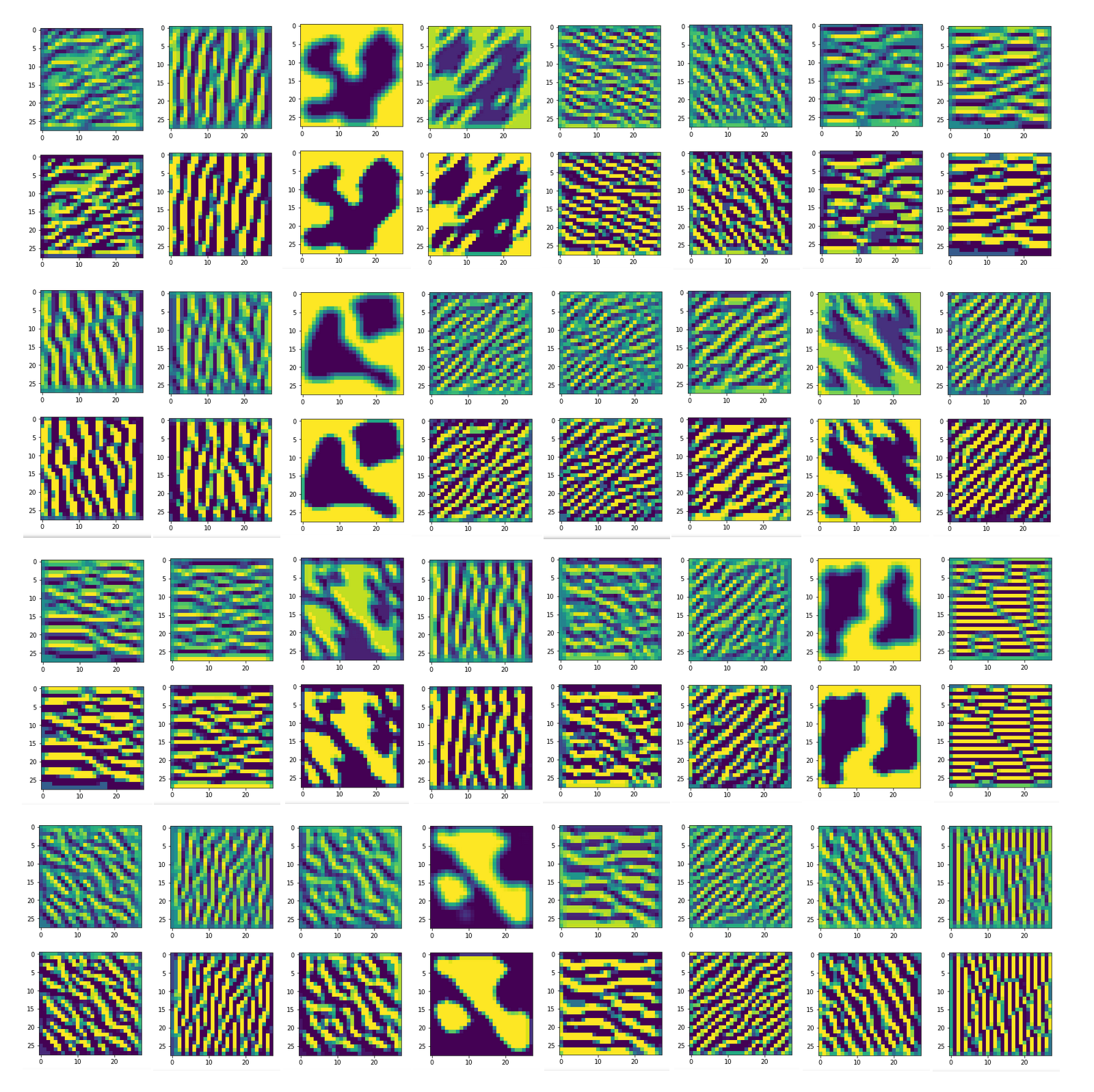
Most of these images were actually derived from one and the same input image.
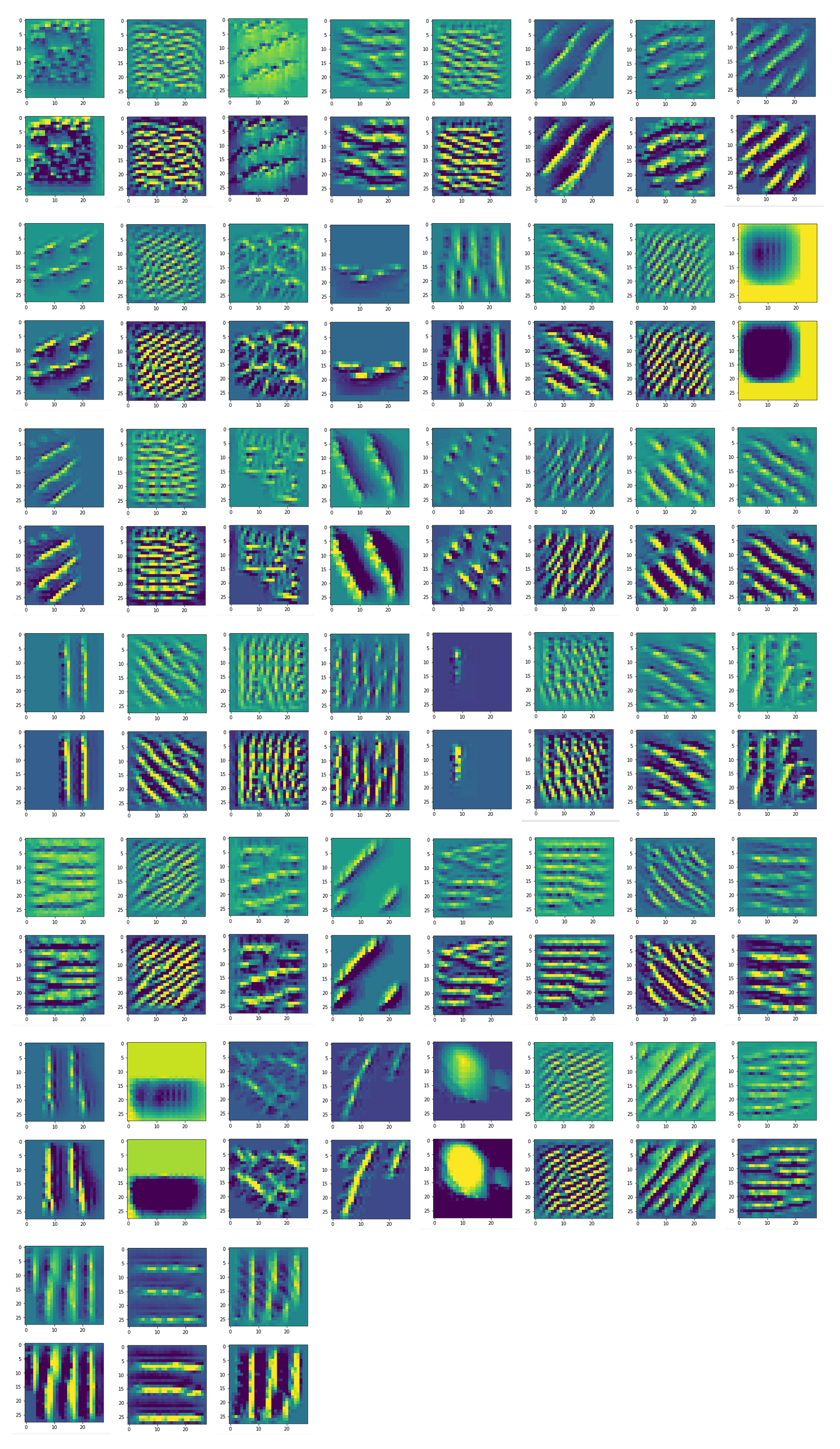
Input image patterns which lead to a maximum
activation of the maps of the convolutional layer Conv2D-2
Layer “Conv2D-2” has 32 maps. With simple fluctuations on the length scale of one to two pixels plus some experiments with pixel value fluctuation son longer scales, I could produce OIP-images for we can easily create OIP-images for 51 of the maps. Experiments for the other 13 maps took to long time; the systematic approach with large scale fluctuations, which we discussed thoroughly in previous articles did not help on layer 2. If you look at the images below, you see that it i more likely that we need specific short and middle-scale fluctuations. However, the amount of possible data combinations is just too big for a systematic investigation.
Conclusion
In the course of the last articles we got a nice overview over the kind of patterns to which the maps of the different convolutional layers of a CNN react to. We are well prepared now to turn back to the question of what the ominous “features” of objects in input images really are. In the meantime have a look at another application of filter visualization in the realm of Deep Dreams, which I recently started to discuss in another article series of this blog. Stay tuned and wear masks to avoid the Corona virus! Stay healthy!
Other (previous) articles in this series
A simple CNN for the MNIST dataset – IV – Visualizing the activation output of convolutional layers and maps
A simple CNN for the MNIST dataset – III – inclusion of a learning-rate scheduler, momentum and a L2-regularizer
A simple CNN for the MNIST datasets – II – building the CNN with Keras and a first test
A simple CNN for the MNIST datasets – I – CNN basics