Als Freelancer hat man seine liebe Not mit der deutschen Last-Minute-DSGVO-Panik. Das Problem ist nicht der Datenschutz an sich; da sind die allgemeinen Anstrengungen eher lobenswert. Das Problem sind vielmehr pauschale Verträge oder Vereinbarungen zur Auftragsverarbeitung, die viele Datenschutzbeauftragte (in ihrer Hilflosigkeit?) uns Freelancern aufdrängen möchten. Dabei spiegeln solche pauschalen Verträge nach meiner Auffassung gerade nicht den Geist der DSGVO wider:
Verkannt wird dabei, dass Datenschutz und Datensicherheit gemeinsame Festlegungen erfordert (s. etwa Art.32 DSGVO). Der Auftraggeber muss nämlich die technischen und organisatorischen Maßnahmen kennen und damit in gewisser Weise auch gutheißen, die Bestandteil eines Vertrages werden sollen. Viele Datenschützer übersehen auch, dass die zu erwartenden personenbezogenen Daten und deren Schutzniveau erstmal definiert werden müssen. Entsprechend inhaltsleer fällt denn auch die Antwort auf die Rückfrage aus, welche personenbezogenen Daten denn in der Zusammenarbeit auftauchen werden.
Man ist als Freelancer also gut beraten, die Schutzbedingungen selbst mit zu definieren – gerade im Geiste der DSGVO, Art. 32, Pkt.1. Das gilt dann u.a. auch für den Austausch von Mails zwischen Auftraggeber und Auftragnehmer.
Das Thema E-Mail ist im Kontext des Datenschutzes für Freelancer durchaus ein kritisches. E-Mails sind von Haus aus mit personenbezogenen Daten behaftet und können weitere schützenswerte Inhalte beinhalten. Hier muss man das zu erreichende Schutzniveau von beiden Seiten also sorgfältig definieren. Dabei muss man einen zwischengeschalteten Provider berücksichtigen – aber natürlich auch die hauseigene E-Mail-Installation. Letztere wird bei Linux-Lovern und -Profis durchaus komplex ausfallen, da der Linux-Anwender/Admin aus vielen vernünftigen Gründen heraus ggf. einen eigenen Mail-Server mit oder ohne Zusammenspiel mit einem Mail-Server bei einem Providern betreiben wird.
Ende-zu-Ende-Verschlüsselung?
Sinnvolle Schutzwege führen bei E-Mail aus meiner Sicht eigentlich immer über Ende-zu-Ende-Verschlüsselung. Kann man die DSGVO also als eine Gelegenheit begreifen, Verschlüsselungspflichten endlich auch für den Auftraggeber zu fixieren? Am besten auf der Basis von OpenPGP? Ich bezweifle aus Jahren eigener schlechter Erfahrung leider, dass alle eure Auftraggeber zu diesem Schritt der Vernunft bereit sein dürften.
Alternative? DE-Mail mit OpenPGP? Ehrlich gesagt: Ich weiß nicht, warum das technisch einfacher sein soll, als gleich selber die Schlüsselverwaltung zu übernehmen – und dabei ganz ohne Browser- oder Client-Plugins auszukommen. DE-Mail ist zudem kostenpflichtig – und man handelt sich ein paar unangenehme Verbindlichkeiten bzgl. der Nutzung ein.
Dennoch ist Mail-Verschlüsselung (ob mit oder ohne DE-Mail) der zu wählende Königsweg.
Nur Verschlüsselung des Übertragungsweges?
Leider fühlen sich viele AGer mit OpenPGP überfordert. Was dann? Nun, meistens haben die Auftraggeber selber E-Mail-Provider – und zumindest erfolgt der Zugang zu den E-Mail-Servern selbiger Provider verschlüsselt. Dito natürlich beim Freelancer. An dieser Stelle erscheint es geboten, als Freelancer einen Auftragsverarbeitungs-Vertrag mit dem Provider abzuschließen, den die meisten Hosting-Provider in Deutschland in pauschaler, aber ggf. hinreichender Weise anbieten.
Schutz unverschlüsselter Mails?
Leider ist man mit der Verschlüsselung des Übertragungsweges als Freelancer nicht aus dem Schneider.
Das erste Thema sind E-Mail-Clients (PCs, Notebooks, ..), die E-Mails in einer unverschlüsselten Umgebung puffern, öffnen oder gar mit Servern synchronisieren (unter Linux etwa über KDE’s Akonadi oder z.B. über Evolutions und Thunderbirds eigene Tools). Auf den Clients bleibt
dann halt viel auf deren meist unverschlüsselten Platten liegen.
Das zweite Thema, das vermutlich gerade Linux-Lover trifft, sind eigene E-Mail-Server im (Home-) Office-LAN. Jeder Freelancer oder auch der Admin eines KMU, der bei seiner Infrastruktur auf Linux setzt, wird aus einer Vielzahl von Gründen früher oder später einen eigenen Mail-Server aufgesetzt und den ggf. an einen Mail-Server bei einem Provider angeschlossen haben. Das gilt im Besonderen dann, wenn noch weitere Mitarbeiter oder Unterauftragnehmer im Spiel sind: Unter Upgrade-, Migrations- und Backup-Gesichtspunkten stellen eigene Mail-Server (trotz der Mühen beim Setup) für den Freelancer letztlich eine Arbeitserleichterung dar. Auf einem solchen Server lagert nun womöglich eine Masse an unverschlüsselten Mails auf unverschlüsselten Festplattenpartitionen. Steht etwa im eigenen (Home-)Office-LAN ein eigener Linux-Mail-Server, stellt sich die Frage wo und wie man die dort auflaufenden E-Mails bei Abwesenheiten/Urlaub von der Wohnung oder seines Office schützt.
Physikalischer Zugangsschutz? Nun, Freelancer werden kaum die Möglichkeit haben, ihre Wohnungen voll zu verriegeln, ohne sich Ärger mit Vermietern einzuhandeln. Wie sichert man sich dann gegen Diebstahl zu schützender Mails im Falle eines Einbruchs während eines Urlaubs ab? Tja – genau mit diesem Problem muss man sich nun ggf. wegen relativ strikter (pauschaler) Auftragsverarbeitungsvereinbarungen mal wieder auseinandersetzen. Das halte ich persönlich für durchaus sinnvoll …
Gefordert ist natürlich erneut Verschlüsselung – diesmal aber von Platten oder Partitionen.
Während Notebooks sowieso durchgehend kryptierte HHDs/SSDs erfordern, ist eine Vollverschlüsselung von Festplatten/ Partitionen bei Servern und umfänglichen Workstations ein viel komplexeres und problematischeres Thema, das auch mit Risiken verbunden ist. Ich nenne nur mal beschädigte Krypto-Header als eines der potentiellen Probleme.
Nehmen wir mal an, man traut sich zu, die Risiken, die mit Kryptographie verbunden sind, zu beherrschen. Wie kann dann für den Linux-Lover ein praktikables Modell für den Schutz unverschlüsselter Mails aussehen? Ich meine, dass drei strategische Elemente zum Ziel führen:
- Abseparation von bestimmten E-Mail-Accounts für Kunden
- Virtualisierung der E-Mail-Server – wie einer E-Mail-Client-Umgebung unter KVM/QEMU
- Verschlüsselung der (Raw-) Partitionen/Volumes, auf denen E-Mail-Server oder aber die Client-Umgebung operieren.
Auf mobilen Laptops/Notebooks ist eine Kryptierung der benutzten Partitionen sowieso Pflicht. Für SSDs ist dabei zu beachten, dass die Verschlüsselung schon im jungfräulichen Zustand erfolgen muss.
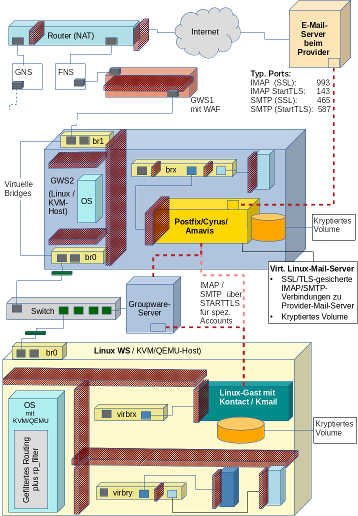
Nun wollen wir die Verschlüsselung aber auch auf Workstation-Clients und Server anwenden. Der E-Mail-Datenverkehr läuft dann meiner Ansicht etwa wie folgt aus:
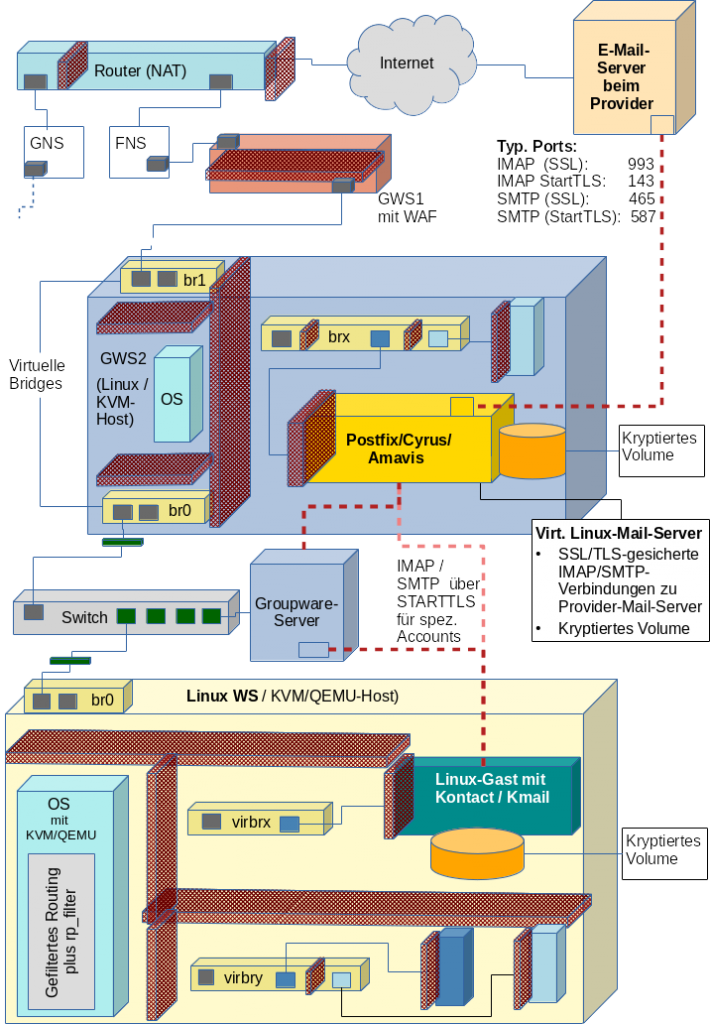
Ein Router mit Perimeter-Firewall übernimmt die Kommunikation mit dem Internet. Er trennt ggf. ein Gastnetz [GNS} von einem Frontend-Segment [FNS]ab. Ein System mit einer Paket-Filter-Firewall und/oder WAF-Firewall trennt weitere nachgelagerte Segmente ab. Ein zweites System GWS2 realisiert einen E-Mail-Server in einer Art sekundärer DMZ. Dieser Server wird entweder direkt von normalen Clients in weiteren Zonen angesprochen (Lösung für “Arme”) oder synchronisiert Mails ggf. mit einem weiteren Groupware-Server in internen Segmenten (Lösung für “Reiche”).
Kennt man sich gut mit Paketfiltern im Kontext virtualisierter
Netze gut aus, kann das angedeutete System “GWS1” ggf. entfallen. Auch der Groupware-Server ist für einen reinen Mail-Betrieb nicht erforderlich.
Die Verschlüsselung der Volumes, die von den unter KVM/QEMU virtualisierten Servern/Clients genutzt werden, kann dabei auf dem Host bereits auf der Ebene einer Linux-“Raw”-Partition oder eines “Raw”-LVM-Volumes genutzt werden. Ich halte in einem solchen Szenario allein aus Performance-Gründen Einiges davon, die Verschlüsselung dem Virtualisierungshost zu überlassen. Sollte jemand dagegen gute Einwände haben, bitte ich um Kontakt per E-Mail ….
Der regelmäßige Austausch von E-Mails, die personenbezogene und andere vertrauliche Daten beinhalten, erfordert mit Auftraggebern ggf. einen Vertrag, der die Art und Qualität personenbezogener Daten definiert, zu erreichende Schutzniveaus festlegt und technische wie organisatorische Maßnahme zu deren Umsetzung regelt.
Eine wichtige Maßnahme bei Freelancern, die keinen hinreichenden Zugangsschutz zu eigenen Systemen garantieren können, erscheint mir dabei die Lagerung der E-Mails auf verschlüsselten Partitionen und Volumes zu sein. Will man nicht gleich alles verschlüsseln können virtualisierte Systeme zum Zuge kommen.
In kommenden Artikel
DSGVO, Freelancer, E-Mails und Umzug KVM-virtualisierter Linux-E-Mail-Server auf verschlüsselte Platten/Partitionen – II
gehe ich zunächst noch einmal auf ein paar Aspekte der DSGVO ein und begründe etwas genauer, warum ein vertragliches Abkommen mit einem Auftraggeber sinnvoll ist. In einem dritten Artikel widme mich dann mal dem Umzug eines Linux-E-Mail-Servers – und dabei speziell dem Umzug einer bereits existierenden virtualisierten Lösung – auf neue, verschlüsselte Partitionen oder LVM-Volumes des Hosts. Entsprechende Arbeiten für Client-Systeme sind dann recht ähnlich.