I continue with my series on Variational Autoencoders [VAEs] and related methods to control the KL-loss.
Variational Autoencoder with Tensorflow – I – some basics
Variational Autoencoder with Tensorflow – II – an Autoencoder with binary-crossentropy loss
Variational Autoencoder with Tensorflow – III – problems with the KL loss and eager execution
Variational Autoencoder with Tensorflow – IV – simple rules to avoid problems with eager execution
Variational Autoencoder with Tensorflow – V – a customized Encoder layer for the KL loss
Variational Autoencoder with Tensorflow – VI – KL loss via tensor transfer and multiple output
Variational Autoencoder with Tensorflow – VII – KL loss via model.add_loss()
Variational Autoencoder with Tensorflow – VIII – TF 2 GradientTape(), KL loss and metrics
Variational Autoencoder with Tensorflow – IX – taming Celeb A by resizing the images and using a generator
Variational Autoencoder with Tensorflow – X – VAE application to CelebA images
VAEs fall into a section of ML which is called “Generative Deep Learning“. The reason is that we can VAEs to create images with contain objects with features of objects learned from training images. One interesting category of such objects are human faces – of different color, with individual expressions and features and hairstyles, seen from different perspectives. One dataset which contains such images is the CelebA dataset.
During the last posts we came so far that we could train a CNN-based Variational Autoencoder [VAE] with images of the CelebA dataset. Even on graphics cards with low VRAM. Our VAE was equipped with a GradientTape()-based method for KL-loss control. We still have to prove that this method works in the expected way:
The distribution of data points (z-points) created by the VAE’s Encoder for training input should be confined to a region around the origin in the latent space (z-space). And neighboring z-points up to a limited distance should result in similar output of the Decoder.
Therefore, we have to look a bit deeper into the results of some VAE-experiments with the CelebA dataset. I have already pointed out why creating rather complex images from arbitrarily chosen points in the latent space is a suitable and good test for a VAE. Please remember that our efforts regarding the KL-loss have to do with the following fact:
not create reasonable images/objects from arbitrarily chosen z-points in the latent space.
This eliminates the use of an AE for creative purposes. A VAE, however, should be able to solve this type of task – at least for z-points in a limited surroundings of the latent space’s origin. Thus, by creating images from randomly selected z-points with the Decoder of a VAE, which has been trained on the CelebA data set, we cover two points:
- Test 1: We test the functionality of the VAE-class, which we have developed and which includes the code for KL-loss handling via TF2’s GradientTape() and Keras’ train_step().
- Test 2: We test the ability of the VAE’s Decoder to create images with convincing human-like face and hairstyle features from random z-points within an area close to the origin of the latent space.
Most of the experiments discussed below follow the same prescription: We take our trained VAE, select some random points in the latent space, feed the z-point-data into the VAE’s Decoder for a prediction and plot the images created on the Decoder’s output side. The Encoder only plays a role when we want to test reconstruction abilities.
For a low dimension z_dim=256 of the latent space we will find that the generated images display human faces reasonably well. But the images appear a bit blurry or unsharp – as if not fully focused. So, we need to discuss what we can do about this point. I will also name some plausible causes for the loss of accuracy in the representation of details.
Afterwards I want to show you that a VAE Decoder reconstructs original images relatively badly from the z-points calculated by the Encoder. At least when one looks at details. A simple AE with a sufficiently high dimension of the latent space performs much better. One may feel disappointed about the reconstruction ability of a VAE. But actually it is the ability of a VAE to forget about details and instead to focus on general features which enables it (the VAE) to create something meaningful from randomly chosen z-points in the latent space.
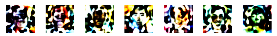
In a last step in this post we are going to look at images created from z-points with a growing distance from the origin of the multidimensional latent space [z-space]. (Distance can be defined by a L2-Euclidean norm). We will see that most z-points which have some z-coordinates above a value of 3 produce fancy images where the face structures get dominated or distorted by background structures learned from CelebA images. This effect was to be expected as the KL-loss enforced a distribution of the z-points which is confined to a region relatively close to the origin. Ideally, this distribution would be characterized by a normal distribution in all coordinates with a sigma of only 1. So, the fact that z-points in the vicinity of the origin of the latent space lead to a construction of images which show recognizable human faces is an indirect proof of the confining impact of the KL-loss on the z-point distribution. In another post I shall deliver data which prove this more directly.
Below I will call the latent space of a (V)AE also z-space.
Characteristics of the VAE tested
Our trained VAE with four Conv2D-layers in the Encoder and 4 corresponding Conv2DTranspose-Layers in the Decoder has the following basic characteristics:
(Encoder-CNN-) filters=(32,64,128,256), kernels=(3,3), stride=2,
reconstruction loss = BCE (binary crossentropy), fact=5.0, z_dim=256
The order of the filter- (= map-) numbers is, of course reversed for the Decoder. The factor fact to scale the KL-loss in comparison to the reconstruction loss was chosen to be fact=5, which led to a 3% contribution of the KL-loss to the total loss during training. The VAE was trained on 170,000 CelebA images with 24 epochs and a small epsilon=0.0005 plus Adam optimizer.
When you perform similar experiments on your own you may notice that the total loss values after around 24 epochs ( > 5015) are significantly higher than those of comparable experiments with a standard AE (4850). This already is an indication that our VAE will not reproduce a similar good match between an image reconstructed by the Decoder in comparison to the original input image fed into the Encoder.
Results for z-points with coordinates taken from a normal distribution around the origin of the latent space
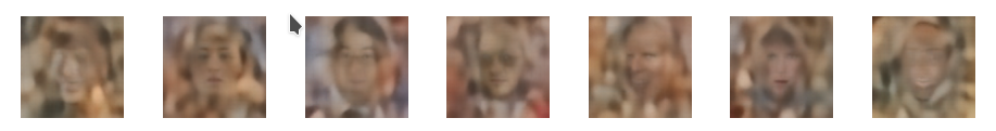
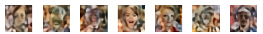
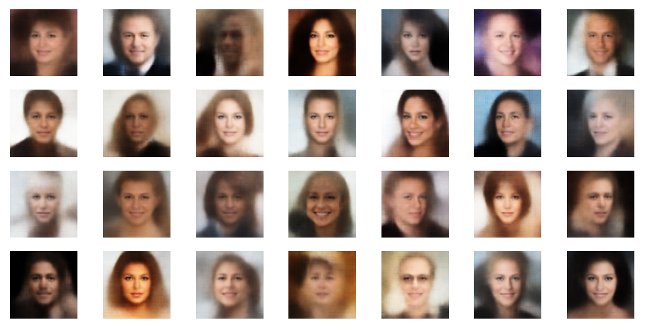
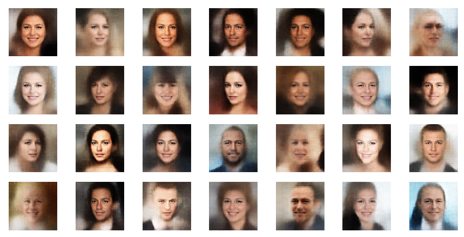
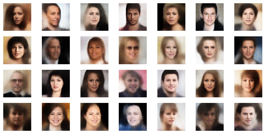
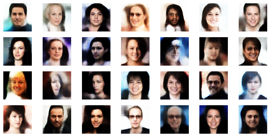
The picture below shows some examples of generated face-images coming from randomly chosen z-points in the vicinity of the z-space’s origin. To calculate the coordinates of such z-points I applied a normal distribution:
z_points = np.random.normal(size = (n_to_show, z_dim)) # n_to_show = 28
So, what do the results for z_dim=256 look like?
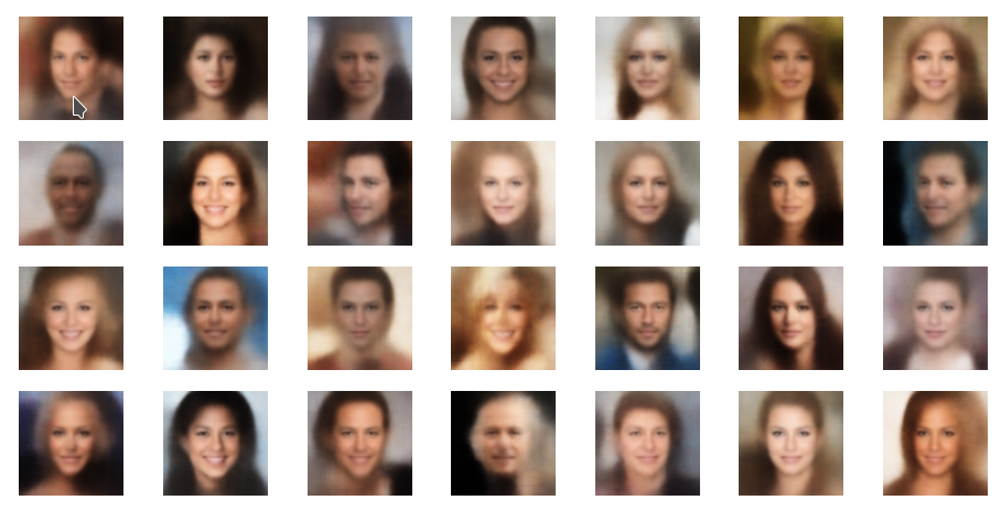
Ok, we get reasonable images of human-like faces. The variations in perspective, face forms and hairstyles are also clearly visible and reflect part of the related variety in the training set. You will find more variations in more images below. So, we take this result as a success! In contrast to a pure AE we DO get something from random z-points which we clearly can interpret as human faces. The whole effort of confining z-points around the origin and at the same time of smearing out z-points with similar content over a region instead of a fixed point-mapping (as in an AE) has paid off. See for comparison:
Autoencoders, latent space and the curse of high dimensionality – I
Unfortunately, the images and their details details appear a bit blurry and not very sharp. Personally, this reminded me of the times when the first CCD-chips with relative low resolution were introduced in cameras and the raw image data looked disappointing as long as we did not apply some sharpening filters. The basic information to enhance details were there, but they had to be used explicitly to improve the plain raw data of the CCD.
The quality in details is about the same as what we see in example images in the book of D.Foster on “Generative Deep Learning”, 2019, O’Reilly. Despite the fact that Foster used a slightly higher resolution of the input images (128x128x3 pixels). The higher input resolution there also led to a higher resolution of the maps of the innermost convolutional layer. Regarding quality see also the images presented in:
https://datagen.tech/guides/image-datasets/celeba/
Enhancement processing of the images ?
Just for fun, I took a screenshot of my result, saved it and applied two different sharpening filters from the ShowFoto program:


Much better! And we do not have the impression that we added some fake information to the images by our post-processing ….
Now I hear already argument saying that such an enhancement should not be done. Frankly, I do not see any reason against post-processing of images created by a VAE-algorithm.
Remember: This is NOT about reproduction quality with respect to originals or a close-to-reality show. This is about generating new mages of human-like faces based on basic features which a VAE-algorithm hopefully has learned from training images. All of what we do with a VAE is creative. And it also comes close to a proof that ML-algorithms based on convolutional layers really can “learn” something about the basic features of objects presented to them. (The learned features are e.g. in the Encoder’s case saved in the sensitivity of the convolutional maps to typical patterns in the input images.)
And as in the case of raw-images of CCD or CMOS camera chips: Sometimes some post-processing is required to utilize the information optimally for sharpness.
Sharpening by PIL’s enhancement functionality
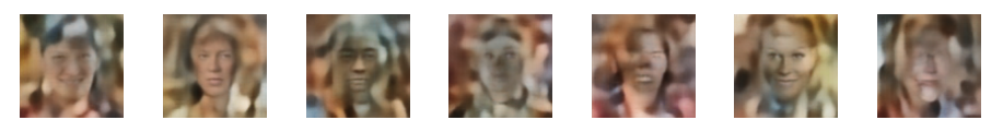
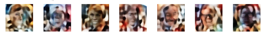
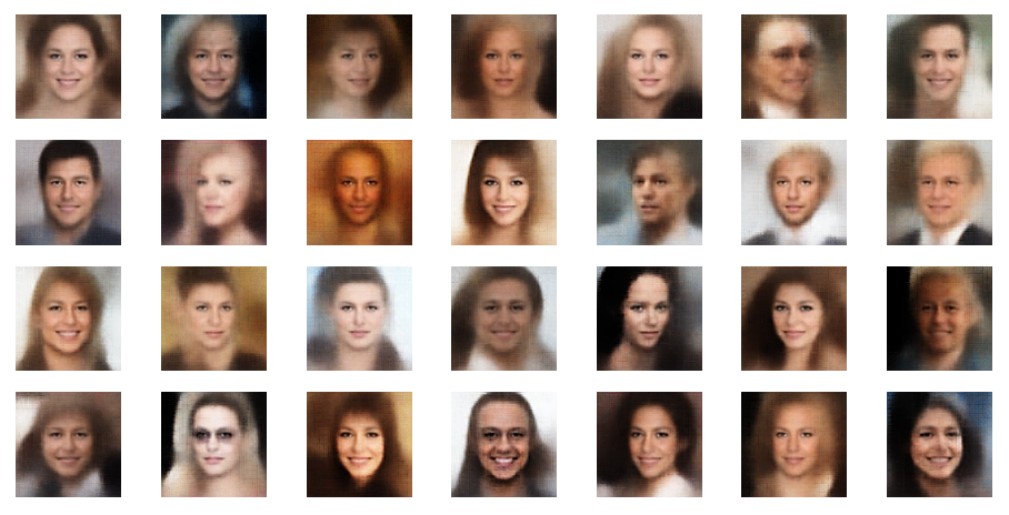
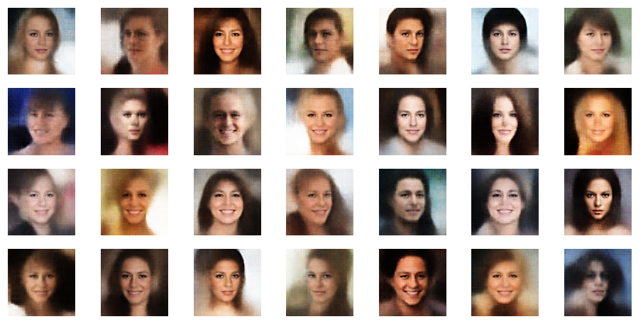
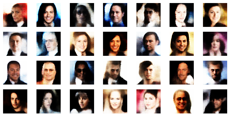
Of course we do not want to produce images in a ML run, take screenshots and sharpen each image individually. We need some tool that fits into the ML process pipeline. The good old PIL library for Python offers sharpening as one of multiple enhancement options for images. The next examples are results from the application of a PIL enhancement procedure:
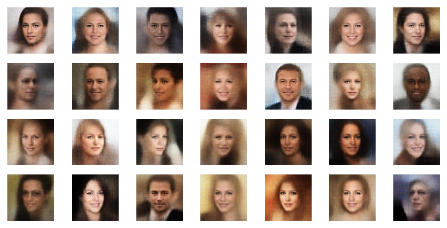
These images look quite OK, too. The basic code fragment I used for each individual image in the above grid:
    # reconst_new is the output from my VAE's Decoder
    ay_img      = reconst_new[i, :,:,:] * 255
    ay_img      = np.asarray(ay_img, dtype="uint8" )
    img_orig    = Image.fromarray(ay_img)
    img_shr_obj = ImageEnhance.Sharpness(img)
    sh_factor   = 7   # Specified Factor for Enhancing Sharpness
    img_sh      = img_shr_obj.enhance(sh_factor)
The sharpening factor I chose was quite high, namely sh_factor = 7.
The effect of PIL’s sharpening factor
Just to further demonstrate the effect of different factors for sharpening by PIL you find some examples below for sh_factor = 0, 3, 6.
sh_factor = 0
sh_factor = 3
sh_factor = 6
Obviously, the enhancement is important to get clearer and sharper images.
However, when you enlarge the images sufficiently enough you see some artifacts in the form of crossing lines. These artifacts are partially already existing in the Decoder’s output, but they are enhanced by the Sharpening mechanism used by PIL (unsharp masking). The artifacts become more pronounced with a growing sh_factor.
Hint: According to ML-literature the use of Upsampling layers instead of Conv2DTranspose layers in the Decoder may reduce such artefacts a bit. I have not yet tried it myself.
Assessment
How do we assess the point of relatively unclear, unsharp images produced by our VAE? What are plausible reasons for the loss of details?
- Firstly, already AEs with a latent space dimension z_dim=256 in general do not reconstruct brilliant images from z-points in the latent space. To get a good reconstruction quality even from an AE which does nothing else than to compress and reconstruct images of a size (96x96x3) z_dim-values > 1000 are required in my experience. More about this in another post in the future.
- A second important aspect is the following: Enforcing a compact distribution of similar images in the latent space via the KL-loss automatically introduces a loss of detail information. The KL-loss is designed to lead to a smear-out effect in z-space. Only basic concepts and features will be kept by the VAE to ensure a similarity of neighboring images. Details will be omitted and “smoothed” out. This has consequences also with respect to sharpness of detail structures. A detail as an eyebrow in a face is to be considered as an average of similar details found for images in the same region of the z-space. This alone brings some loss of clarity with it.
- Thirdly, a simple (V)AE based on some directly connected Conv2D-layers has limited capabilities in general. The reason is that we systematically reduce resolution whilst information is propagated from one Conv2D layer to the next neighboring one. Remember that we use a stride > 2 or pooling layers to cover filters on larger image scales. Due to this information processing a convolutional network automatically suppresses details in its inner layers – their resolution shrinks with growing distance from the input layer. In later posts of this blog we shall see that using ResNets instead of CNNs in the Encoder and Decoder already helps a bit regarding the reconstruction of clearer images. The correlation between details and large scale information is better kept up there than in CNNs.
Regarding the first point one may think of increasing z_dim. This may not be the best idea. It contradicts the whole idea of a VAE which at its core is a reduction of the degrees of freedom for z-points. For a higher dimensional space we may have to raise the ratio of KL-loss to reconstruction loss even further.
Regarding the third point: Of course it would also help to increase kernel sizes for the first two Conv2D layers and the number of maps there. A higher resolution of the input images would also be of advantage. Both methods may, however, conflict with your VRAM or GPU time limits.
If the second point were true then reduction of fact in our models, which controls the ration of KL-loss to reconstruction loss, would lead to a better image quality. In this case we are doomed to find an optimal value for fact – satisfying both the need for generalization and clarity of details in our images. You cannot have both … here we see a basic problem related to VAEs and the creation of realistic images. Actually, I tried this out – the effect is there, but the gain actually is not worth the effort. And for too small values of fact we eventually loose the ability to create reasonable images from arbitrary z-points at all.
All in all post-processing appears to be a simple and effective method to get images with somewhat sharper details.
Hint: If you want to create images of artificially generated faces with a really high quality, you have to turn to GANs.
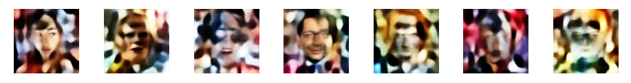
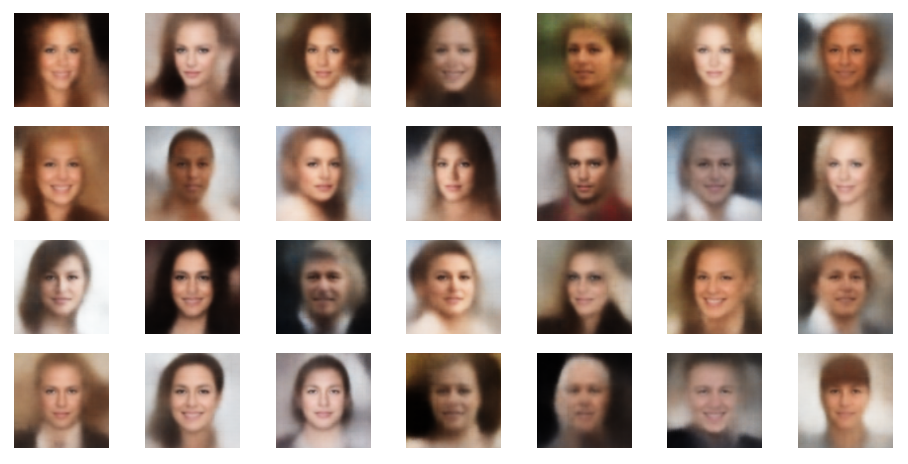
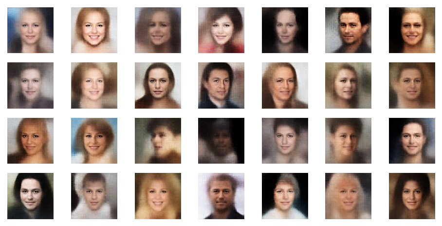
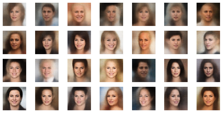
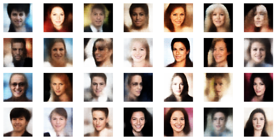
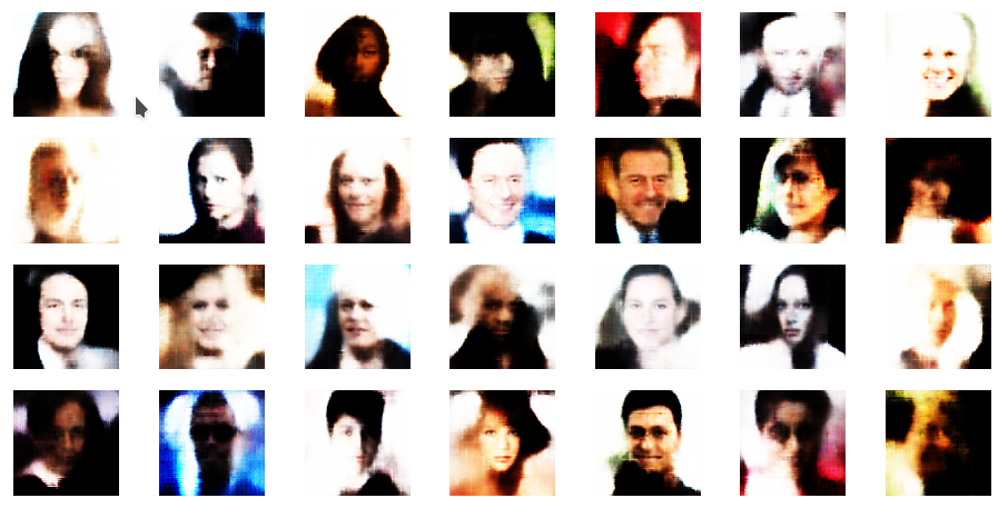
Further examples – with PIL sharpening
In this example you see that not all points give you good images of faces. The z-point of the middle image in the second to last of the first illustration below has a relatively high distance from the origin. The higher the distance from the origin in z-space the weirder the images get. We shall see this below in a more systematic way.
Reconstruction quality of a VAE vs. an AE – or the “female” side of myself
If I were not afraid of copy and personal rights aspects of using CelebA images directly I could show you now a comparison of the the reconstruction ability of an AE in comparison to a VAE. You find such a comparison, though a limited one, by looking at some images in the book of D. Foster.
To avoid any problems I just tried to work with an image of myself. Which really gave me a funny result.
A plain Autoencoder with
- an extended latent space dimension of z_dim = 1600,
- a reasonable convolutional filter sequence of (64, 64, 128, 128)
- a stride value of stride=2
- and kernels ((5,5),(5,5),(3,3),(3,3))
is well able to reproduce many detailed features one’s face after a training on 80,000 CelebA images. Below see the result for an image of myself after 24 training epochs of such an AE:

The left image is the original, the right one the reconstruction. The latter is not perfect, but many details have been reproduced. Please note that the trained AE never had seen an image of myself before. For biometric analysis the reproduction would probably be sufficient.
Ok, so much about an AE and a latent space with a relatively high dimension. But what does a VAE think of me?
With fact = 5.0, filters like (32,64,128,256), (3,3)-kernels, z_dim=256 and after 18 epochs with 170,000 training images of CelebA my image really got a good cure:
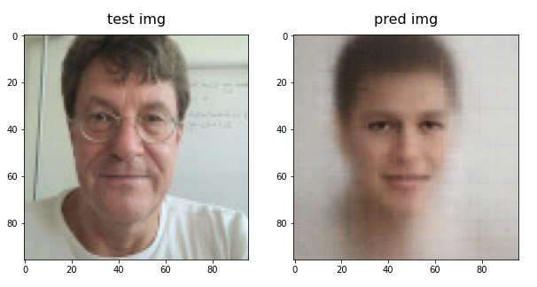
My wife just laughed and said: Well, now in the age of 64 at least an AI has found something soft and female in you … Well, had the CelebA included many faces of heavy metal figures the results would have looked differently. I bet …
So with generative VAEs we obviously pay a price: Details are neglected in favor of very general face features and hairstyle aspects. And we loose sharpness. Which is good if you have wrinkles. Good for me and the celebrities, too. 🙂
However, I recommend anybody who wants to study VAEs to check the reproduction quality for CelebA test images (not from the training set). You will see the generalization effect for a broader range of images. And, of course, a better reproduction with smaller values for the ratio of the KL-loss to the reconstruction loss. However, for too small values of fact you will not be able to create realistic face images at all from arbitrary z-points – even if you choose them to be relatively close to the origin of the latent space.
Dependency of the creation of reasonable images on the distance from the origin
In another post in this blog I have discussed why we need VAEs at all if we want to reconstruct reasonable face images from randomly picked points in the latent space. See:
Autoencoders, latent space and the curse of high dimensionality – I
I think the reader is meanwhile convinced that VAEs do a reasonably good job to create images from randomly chosen z-points. But all of the above images were taken from z-points calculated with the help of a function assuming a normal distribution in the z-space coordinates. The width of the resulting distribution around the origin is of course rather limited. Most points lie within a 3 sigma distance around the origin. This is OK as we have put a lot of effort into the KL-loss to force the z-points to approach such a normal distribution around the origin of the latent space.
But what happens if and when we increase the distance of our random z-points from the origin? An easy way to investigate this is to create the z-points with a function that creates the coordinates randomly, but equally distributed in an interval ]0,limit]. The chance that at least one of the coordinates gets a high value is rather big then. This in turn ensures relatively high radius values (in terms of an L2-distance norm).
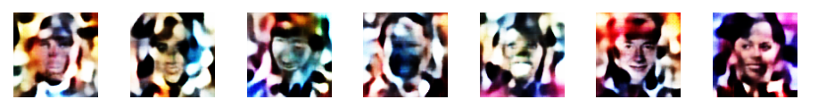
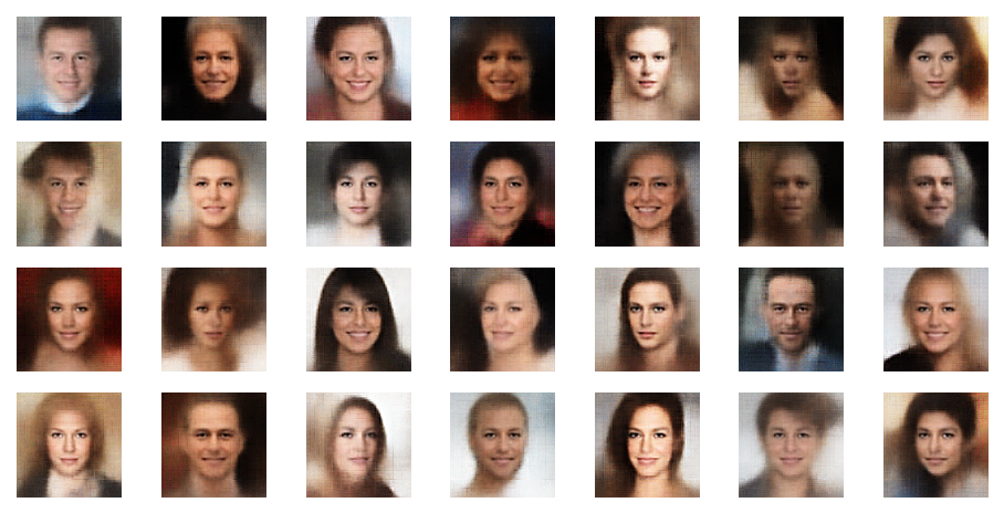
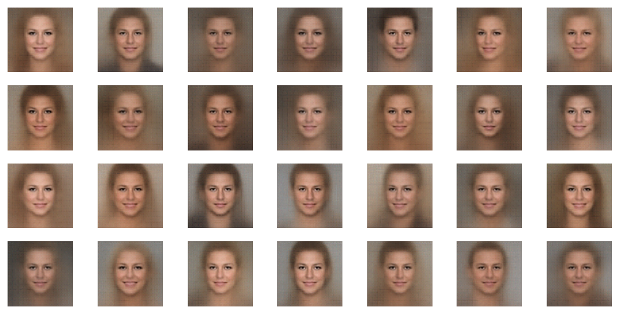
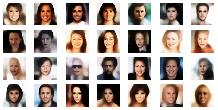
Below you find the results for z-points created by the function random.uniform:
r_limit = 1.5
l_limit = -r_limit
znew = np.random.uniform(l_limit, r_limit, size = (n_to_show, z_dim))
r_limit is varied as indicated:
r_limit = 0.5
r_limit = 1.0

r_limit = 1.5
r_limit = 2.0
r_limit = 2.5
r_limit = 3.0
r_limit = 3.5
r_limit = 5.0
r_limit = 8.0
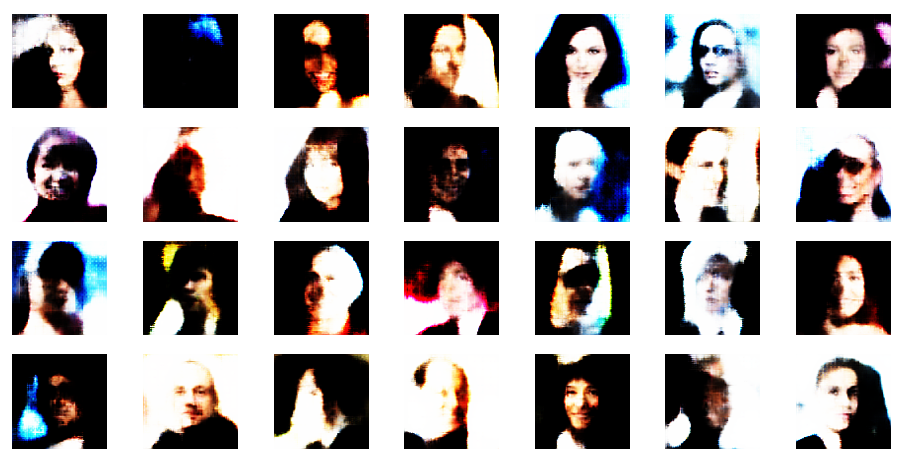
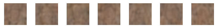
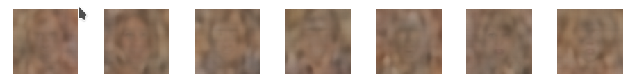
Well, this proves that we get reasonable images only up to a certain distance from the origin – and only in certain areas or pockets of the z-space at higher radii.
Another notable aspect is the fact that the background variations are completely smoothed out a low distances from the origin. But they get dominant in the outer regions of the z-space. This is consistent with the fact that we need more information to distinguish various background shapes, forms and colors than basic face patterns. Note also that the faces appear relatively homogeneous for r_limit = 0.5. The farther we are away from the origin the larger the volumes to cover and distinguish certain features of the training images become.
Conclusion
Our VAE with the GradientTape()-mechanism for the control of the KL-loss seems to do its job. In contrast to a pure AE the smear-out effect of the KL-loss allows now for the creation of images with interpretable contents from arbitrary z-points via the VAE’s Decoder – as long as the selected z-points are not too far away from the z-space’s origin. Thus, by indirect evidence we can conclude that the z-points for training images of the CelebA dataset were distributed and at the same time confined around the origin. The strongest indication came from the last series of images. But we pay a price: The reconstruction abilities of a VAE are far below those of AEs. A relatively low number of dimensions of the latent space helps with an effective confinement of the z-points. But it leads to a significant loss in detail sharpness of the generated images, too. However, part of this effect can be compensated by the application of standard procedures for image enhancemnet.
In the next post
Variational Autoencoder with Tensorflow – XII – save some VRAM by an extra Dense layer in the Encoder
I will discuss a simple trick to reduce the VRAM consumption of the Encoder. In a further post we shall then analyze the confinement of the z-point distribution with the help of more explicit data.
And let us all who praise freedom not forget:
The worst fascist, war criminal and killer living today is the Putler. He must be isolated at all levels, be denazified and sooner than later be imprisoned. An aggressor who orders the bombardment of civilian infrastructure, civilian buildings, schools and hospitals with drones bought from other anti-democrats and women oppressors puts himself in the darkest and most rotten corner of human history.