Variational Autoencoder with Tensorflow – XII – save some VRAM by an extra Dense layer in the Encoder

I continue with my series on Variational Autoencoders [VAEs] and related methods to control the KL-loss.

Variational Autoencoder with Tensorflow 2.8 – I – some basics
Variational Autoencoder with Tensorflow 2.8 – II – an Autoencoder with binary-crossentropy loss
Variational Autoencoder with Tensorflow 2.8 – III – problems with the KL loss and eager execution
Variational Autoencoder with Tensorflow 2.8 – IV – simple rules to avoid problems with eager execution
Variational Autoencoder with Tensorflow 2.8 – V – a customized Encoder layer for the KL loss
Variational Autoencoder with Tensorflow 2.8 – VI – KL loss via tensor transfer and multiple output
Variational Autoencoder with Tensorflow 2.8 – VII – KL loss via model.add_loss()
Variational Autoencoder with Tensorflow 2.8 – VIII – TF 2 GradientTape(), KL loss and metrics
Variational Autoencoder with Tensorflow 2.8 – IX – taming Celeb A by resizing the images and using a generator
Variational Autoencoder with Tensorflow 2.8 – X – VAE application to CelebA images
Variational Autoencoder with Tensorflow 2.8 – XI – image creation by a VAE trained on CelebA

After having successfully trained a VAE with CelebA data, we have shown that our VAE can afterward create images with human-like looking faces from statistically selected data points (z-points) in its latent space. We still have to analyze the confinement of the z-point distribution due to the KL-loss a bit in more depth. But before we turn to this topic I want to briefly discuss an option to reduce the VRAM requirements of the VAE’s Encoder.

Limited VRAM – a problem for ML training runs on older graphics cards

In my opinion exploring the field of Machine Learning on a PC should not be limited to people who can afford a state of the art graphics card with a lot of VRAM. One could use Google’s Colab – but … I do not want to go into tax and personal data politics here. I really miss an EU-wide platform that offers services like Google Colab.

Anyway, a reduction of VRAM consumption may be decisive to be able to perform training runs for CNN-based VAEs on older graphic cards . Not only concerning VRAM limits but also regarding computational time: The less VRAM the weight parameters of our VAE models require the bigger we can size the batches the GPU operates on and the more CPU time we may potentially save. At least in principle. Therefore, we should consider the amount of trainable parameters of a neural network model and reduce them if possible.

The number of parameters depends heavily on the connections to the mu and logvar-layer of the Encoder

When you print out the layer structure and related parameters of a VAE (see below) you will find that the Encoder requires more parameters than the Decoder. Around twice as many. A closer look reveals:

It is the transition from the convolutional part of the Encoder to its Dense layers for mu and logvar which plays an important role for the number of weight parameters.

For a layer structure comprising 4 Conv2D layers, related filters=(32,64,128,256) and an input image size of (96,96,3) pixels we arrive at a Flatten-layer of 9216 neurons at the end of the convolutional part of the Encoder. For z_dim = 512 the direct connections from the Flatten-layer to both the mu- and logvar-layers lead to more the 9.4 million (float32) parameters for the Encoder. This is the absolutely dominant part of all required 9.83 million parameters of the Encoder. In contrast the Decoder part requires a total of 5.1 million parameters, only.

Encoder

Decoder

This is due to the fact that the flattened layer supplies input to two connected layers before output is created by yet another layer. In the Decoder, instead, only one layer, namely the input layer is connected to the flattened layer ahead of the first Conv2DTranspose layer.

In the case of z_dim=256 we arrive at around half of the parameters, i.e. 4.9 million parameters for the Encoder and around 2.76 million for the Decoder.

It is obvious that the existence of two layers for the variational parameters inside the Encoder is the source of the high parameter number on the Encoder side.

Would a reduction of convolutional layers help to reduce the weight parameters?

A reduction of Conv2D-layers in the Encoder would of course reduce the parameters for the weights between the convolutional layers. But turning to only three convolutional layers whilst keeping up a stride value of stride=2 for all filters would raise the already dominant number of parameters after the flattened layer by a factor of 4!

So, one has to work with a delicate balance between the number of convolutional layers and the eventual number of maps at the innermost layer and the size of these maps. They determine the number of neurons and related weights on the flattening layer:

From the perspective of a low total number of parameters you should consider higher stride values when reducing the number of Conv2D-layers.

On the other hand side using more than 4 convolutional layers would reduce the resolution of the maps of the innermost Conv2D layer below a usable threshold for reasonable mu and logvar values.

Off topic remark: All in all it seems to be reasonable also to think about ResNets of low depth instead of plain CNNs to keep weight numbers under control.

An intermediate dense layer ahead of the mu- and logvar-layers of the Encoder?

The reader who followed the posts in this series may have looked at the recipe which F. Chollet has discussed in his Keras documentation on VAEs. See:
https://keras.io/ examples/ generative/vae/.

There is an element in Chollet’s Encoderstructure which one easily can overlook at first sight. In his example for the MNIST dataset Chollet adds an intermediate Dense layer between the Flatten-layer and the layers for mu and logvar.

...
x = layers.Flatten()(x)
x = layers.Dense(16, activation="relu")(x)
z_mean = layers.Dense(latent_dim, name="z_mean")(x)
z_log_var = layers.Dense(latent_dim, name="z_log_var")(x)
...

In the special case of MNIST an intermediate layer seems appropriate for bridging the gap between an input dimension of 784 to z_dim = 2. You do not expect major problems to arise from such a measure.

But: This intermediate layer introduced by Chollet also has the advantage of reducing the total number of trainable parameters substantially.

We could try something similar for our network. But here we have to be a bit more careful as we work in a latent space of much higher dimensions, typically with z_dim >= 256. Here we are in dilemma as we want to keep the intermediate dimension relatively high for using as much information as possible coming from the maps of the last Conv2D-layers. A fair compromise seems to be to use at least the dimension of the mu and varlog-layers, namely z_dim.

For z_dim=256 an additional Dense layer of the same size would reduce the total number of Encoder parameters from 5.11 million to 2.88 million.

If we took the dimension of the intermediate layer to be 384 we would still go down with the total Encoder parameters to 4.13 million. So an additional Dense layer really saves us some VRAM.

Images constructed by a VAE model with an additional Dense layer in the Encoder

Will an additional dense layer have a negative impact on our VAE’s ability to create images from randomly chosen z-points in the latent space?

Let us try it out. To include an option for an additional Dense layer in the Encoder related part of our class “MyVariationalAutoencoder()” is a pretty simple task. I leave this to the reader. Note that if we choose the dimension of the additional Dense layer to be exactly z_dim there is no need to change the reconstruction logic and layer structure of the Decoder. Also for other choices for the size of the Dense layer I would refrain from changing the Decoder.

I used z_dim=256 for the extra layer’s size. Then I repeated the experiments described in my last post. Some results for random z-points picked from a normal distribution in all coordinates are shown below:

So we see that from the generative point of view an extra Dense layer does not hurt too much.

What have we gained?

First and foremost:

We found a simple method to reduce the VRAM consumption of the Encoder.

But I have to admit that this method did NOT save any GPU time during training as long as I kept the size of image batches equally big as before (128). The reason is:

Due to the extra layer more matrix operations have to be performed than before, although some of matrixes becae smaller. On my old graphics card a full epoch with 170,000 (96×96) images takes around 120 secs – with or without an extra Encoder layer. Unfortunately, increasing the size of the batches the DataImageGenerator feeds into the GPU from 128 images to 256 did not change the required GPU time very much. More tests showed that a size of 128 already gave me an optimal turnaround time per epoch on my old graphics card (960 GTX).

Conclusion

An extra intermediate Dense layer between the Flatten-layer and the mu- and logvar-layers of the Encoder can help us to save some VRAM during the training of a VAE. Such a layer does not lead to a visible reduction of the quality of VAE-generated images from randomly selected points in the latent-space.

In the next post of this series
Variational Autoencoder with Tensorflow 2.8 – XIII – Does a VAE with tiny KL-loss behave like an AE? And if so, why?
we will compare a VAE with only a tiny contribution of KL-loss to the total loss with a corresponding AE. We shall investigate their similarity regarding their z-point distributions. This will give us a solid basis to investigate the impact of higher KL-loss values on the latent space in more detail afterwards.

Variational Autoencoder with Tensorflow – XI – image creation by a VAE trained on CelebA

I continue with my series on Variational Autoencoders [VAEs] and related methods to control the KL-loss.

Variational Autoencoder with Tensorflow – I – some basics
Variational Autoencoder with Tensorflow – II – an Autoencoder with binary-crossentropy loss
Variational Autoencoder with Tensorflow – III – problems with the KL loss and eager execution
Variational Autoencoder with Tensorflow – IV – simple rules to avoid problems with eager execution
Variational Autoencoder with Tensorflow – V – a customized Encoder layer for the KL loss
Variational Autoencoder with Tensorflow – VI – KL loss via tensor transfer and multiple output
Variational Autoencoder with Tensorflow – VII – KL loss via model.add_loss()
Variational Autoencoder with Tensorflow – VIII – TF 2 GradientTape(), KL loss and metrics
Variational Autoencoder with Tensorflow – IX – taming Celeb A by resizing the images and using a generator
Variational Autoencoder with Tensorflow – X – VAE application to CelebA images

VAEs fall into a section of ML which is called “Generative Deep Learning“. The reason is that we can VAEs to create images with contain objects with features of objects learned from training images. One interesting category of such objects are human faces – of different color, with individual expressions and features and hairstyles, seen from different perspectives. One dataset which contains such images is the CelebA dataset.

During the last posts we came so far that we could train a CNN-based Variational Autoencoder [VAE] with images of the CelebA dataset. Even on graphics cards with low VRAM. Our VAE was equipped with a GradientTape()-based method for KL-loss control. We still have to prove that this method works in the expected way:

The distribution of data points (z-points) created by the VAE’s Encoder for training input should be confined to a region around the origin in the latent space (z-space). And neighboring z-points up to a limited distance should result in similar output of the Decoder.

Therefore, we have to look a bit deeper into the results of some VAE-experiments with the CelebA dataset. I have already pointed out why creating rather complex images from arbitrarily chosen points in the latent space is a suitable and good test for a VAE. Please remember that our efforts regarding the KL-loss have to do with the following fact:

not create reasonable images/objects from arbitrarily chosen z-points in the latent space.

This eliminates the use of an AE for creative purposes. A VAE, however, should be able to solve this type of task – at least for z-points in a limited surroundings of the latent space’s origin. Thus, by creating images from randomly selected z-points with the Decoder of a VAE, which has been trained on the CelebA data set, we cover two points:

  • Test 1: We test the functionality of the VAE-class, which we have developed and which includes the code for KL-loss handling via TF2’s GradientTape() and Keras’ train_step().
  • Test 2: We test the ability of the VAE’s Decoder to create images with convincing human-like face and hairstyle features from random z-points within an area close to the origin of the latent space.

Most of the experiments discussed below follow the same prescription: We take our trained VAE, select some random points in the latent space, feed the z-point-data into the VAE’s Decoder for a prediction and plot the images created on the Decoder’s output side. The Encoder only plays a role when we want to test reconstruction abilities.

For a low dimension z_dim=256 of the latent space we will find that the generated images display human faces reasonably well. But the images appear a bit blurry or unsharp – as if not fully focused. So, we need to discuss what we can do about this point. I will also name some plausible causes for the loss of accuracy in the representation of details.

Afterwards I want to show you that a VAE Decoder reconstructs original images relatively badly from the z-points calculated by the Encoder. At least when one looks at details. A simple AE with a sufficiently high dimension of the latent space performs much better. One may feel disappointed about the reconstruction ability of a VAE. But actually it is the ability of a VAE to forget about details and instead to focus on general features which enables it (the VAE) to create something meaningful from randomly chosen z-points in the latent space.

In a last step in this post we are going to look at images created from z-points with a growing distance from the origin of the multidimensional latent space [z-space]. (Distance can be defined by a L2-Euclidean norm). We will see that most z-points which have some z-coordinates above a value of 3 produce fancy images where the face structures get dominated or distorted by background structures learned from CelebA images. This effect was to be expected as the KL-loss enforced a distribution of the z-points which is confined to a region relatively close to the origin. Ideally, this distribution would be characterized by a normal distribution in all coordinates with a sigma of only 1. So, the fact that z-points in the vicinity of the origin of the latent space lead to a construction of images which show recognizable human faces is an indirect proof of the confining impact of the KL-loss on the z-point distribution. In another post I shall deliver data which prove this more directly.

Below I will call the latent space of a (V)AE also z-space.

Characteristics of the VAE tested

Our trained VAE with four Conv2D-layers in the Encoder and 4 corresponding Conv2DTranspose-Layers in the Decoder has the following basic characteristics:

(Encoder-CNN-) filters=(32,64,128,256), kernels=(3,3), stride=2,
reconstruction loss = BCE (binary crossentropy), fact=5.0, z_dim=256

The order of the filter- (= map-) numbers is, of course reversed for the Decoder. The factor fact to scale the KL-loss in comparison to the reconstruction loss was chosen to be fact=5, which led to a 3% contribution of the KL-loss to the total loss during training. The VAE was trained on 170,000 CelebA images with 24 epochs and a small epsilon=0.0005 plus Adam optimizer.

When you perform similar experiments on your own you may notice that the total loss values after around 24 epochs ( > 5015) are significantly higher than those of comparable experiments with a standard AE (4850). This already is an indication that our VAE will not reproduce a similar good match between an image reconstructed by the Decoder in comparison to the original input image fed into the Encoder.

Results for z-points with coordinates taken from a normal distribution around the origin of the latent space

The picture below shows some examples of generated face-images coming from randomly chosen z-points in the vicinity of the z-space’s origin. To calculate the coordinates of such z-points I applied a normal distribution:

z_points = np.random.normal(size = (n_to_show, z_dim)) # n_to_show = 28

So, what do the results for z_dim=256 look like?

Ok, we get reasonable images of human-like faces. The variations in perspective, face forms and hairstyles are also clearly visible and reflect part of the related variety in the training set. You will find more variations in more images below. So, we take this result as a success! In contrast to a pure AE we DO get something from random z-points which we clearly can interpret as human faces. The whole effort of confining z-points around the origin and at the same time of smearing out z-points with similar content over a region instead of a fixed point-mapping (as in an AE) has paid off. See for comparison:
Autoencoders, latent space and the curse of high dimensionality – I

Unfortunately, the images and their details details appear a bit blurry and not very sharp. Personally, this reminded me of the times when the first CCD-chips with relative low resolution were introduced in cameras and the raw image data looked disappointing as long as we did not apply some sharpening filters. The basic information to enhance details were there, but they had to be used explicitly to improve the plain raw data of the CCD.

The quality in details is about the same as what we see in example images in the book of D.Foster on “Generative Deep Learning”, 2019, O’Reilly. Despite the fact that Foster used a slightly higher resolution of the input images (128x128x3 pixels). The higher input resolution there also led to a higher resolution of the maps of the innermost convolutional layer. Regarding quality see also the images presented in:
https://datagen.tech/guides/image-datasets/celeba/

Enhancement processing of the images ?

Just for fun, I took a screenshot of my result, saved it and applied two different sharpening filters from the ShowFoto program:

Much better! And we do not have the impression that we added some fake information to the images by our post-processing ….

Now I hear already argument saying that such an enhancement should not be done. Frankly, I do not see any reason against post-processing of images created by a VAE-algorithm.

Remember: This is NOT about reproduction quality with respect to originals or a close-to-reality show. This is about generating new mages of human-like faces based on basic features which a VAE-algorithm hopefully has learned from training images. All of what we do with a VAE is creative. And it also comes close to a proof that ML-algorithms based on convolutional layers really can “learn” something about the basic features of objects presented to them. (The learned features are e.g. in the Encoder’s case saved in the sensitivity of the convolutional maps to typical patterns in the input images.)

And as in the case of raw-images of CCD or CMOS camera chips: Sometimes some post-processing is required to utilize the information optimally for sharpness.

Sharpening by PIL’s enhancement functionality

Of course we do not want to produce images in a ML run, take screenshots and sharpen each image individually. We need some tool that fits into the ML process pipeline. The good old PIL library for Python offers sharpening as one of multiple enhancement options for images. The next examples are results from the application of a PIL enhancement procedure:

These images look quite OK, too. The basic code fragment I used for each individual image in the above grid:

    # reconst_new is the output from my VAE's Decoder 
    ay_img      = reconst_new[i, :,:,:] * 255
    ay_img      = np.asarray(ay_img, dtype="uint8" )
    img_orig    = Image.fromarray(ay_img)
    img_shr_obj = ImageEnhance.Sharpness(img)
    sh_factor   = 7   # Specified Factor for Enhancing Sharpness
    img_sh      = img_shr_obj.enhance(sh_factor)

The sharpening factor I chose was quite high, namely sh_factor = 7.

The effect of PIL’s sharpening factor

Just to further demonstrate the effect of different factors for sharpening by PIL you find some examples below for sh_factor = 0, 3, 6.

sh_factor = 0

sh_factor = 3

sh_factor = 6

Obviously, the enhancement is important to get clearer and sharper images.
However, when you enlarge the images sufficiently enough you see some artifacts in the form of crossing lines. These artifacts are partially already existing in the Decoder’s output, but they are enhanced by the Sharpening mechanism used by PIL (unsharp masking). The artifacts become more pronounced with a growing sh_factor.
Hint: According to ML-literature the use of Upsampling layers instead of Conv2DTranspose layers in the Decoder may reduce such artefacts a bit. I have not yet tried it myself.

Assessment

How do we assess the point of relatively unclear, unsharp images produced by our VAE? What are plausible reasons for the loss of details?

  1. Firstly, already AEs with a latent space dimension z_dim=256 in general do not reconstruct brilliant images from z-points in the latent space. To get a good reconstruction quality even from an AE which does nothing else than to compress and reconstruct images of a size (96x96x3) z_dim-values > 1000 are required in my experience. More about this in another post in the future.
  2. A second important aspect is the following: Enforcing a compact distribution of similar images in the latent space via the KL-loss automatically introduces a loss of detail information. The KL-loss is designed to lead to a smear-out effect in z-space. Only basic concepts and features will be kept by the VAE to ensure a similarity of neighboring images. Details will be omitted and “smoothed” out. This has consequences also with respect to sharpness of detail structures. A detail as an eyebrow in a face is to be considered as an average of similar details found for images in the same region of the z-space. This alone brings some loss of clarity with it.
  3. Thirdly, a simple (V)AE based on some directly connected Conv2D-layers has limited capabilities in general. The reason is that we systematically reduce resolution whilst information is propagated from one Conv2D layer to the next neighboring one. Remember that we use a stride > 2 or pooling layers to cover filters on larger image scales. Due to this information processing a convolutional network automatically suppresses details in its inner layers – their resolution shrinks with growing distance from the input layer. In later posts of this blog we shall see that using ResNets instead of CNNs in the Encoder and Decoder already helps a bit regarding the reconstruction of clearer images. The correlation between details and large scale information is better kept up there than in CNNs.

Regarding the first point one may think of increasing z_dim. This may not be the best idea. It contradicts the whole idea of a VAE which at its core is a reduction of the degrees of freedom for z-points. For a higher dimensional space we may have to raise the ratio of KL-loss to reconstruction loss even further.

Regarding the third point: Of course it would also help to increase kernel sizes for the first two Conv2D layers and the number of maps there. A higher resolution of the input images would also be of advantage. Both methods may, however, conflict with your VRAM or GPU time limits.

If the second point were true then reduction of fact in our models, which controls the ration of KL-loss to reconstruction loss, would lead to a better image quality. In this case we are doomed to find an optimal value for fact – satisfying both the need for generalization and clarity of details in our images. You cannot have both … here we see a basic problem related to VAEs and the creation of realistic images. Actually, I tried this out – the effect is there, but the gain actually is not worth the effort. And for too small values of fact we eventually loose the ability to create reasonable images from arbitrary z-points at all.

All in all post-processing appears to be a simple and effective method to get images with somewhat sharper details.
Hint: If you want to create images of artificially generated faces with a really high quality, you have to turn to GANs.

Further examples – with PIL sharpening

In this example you see that not all points give you good images of faces. The z-point of the middle image in the second to last of the first illustration below has a relatively high distance from the origin. The higher the distance from the origin in z-space the weirder the images get. We shall see this below in a more systematic way.

Reconstruction quality of a VAE vs. an AE – or the “female” side of myself

If I were not afraid of copy and personal rights aspects of using CelebA images directly I could show you now a comparison of the the reconstruction ability of an AE in comparison to a VAE. You find such a comparison, though a limited one, by looking at some images in the book of D. Foster.

To avoid any problems I just tried to work with an image of myself. Which really gave me a funny result.

A plain Autoencoder with

  • an extended latent space dimension of z_dim = 1600,
  • a reasonable convolutional filter sequence of (64, 64, 128, 128)
  • a stride value of stride=2
  • and kernels ((5,5),(5,5),(3,3),(3,3))

is well able to reproduce many detailed features one’s face after a training on 80,000 CelebA images. Below see the result for an image of myself after 24 training epochs of such an AE:

The left image is the original, the right one the reconstruction. The latter is not perfect, but many details have been reproduced. Please note that the trained AE never had seen an image of myself before. For biometric analysis the reproduction would probably be sufficient.

Ok, so much about an AE and a latent space with a relatively high dimension. But what does a VAE think of me?
With fact = 5.0, filters like (32,64,128,256), (3,3)-kernels, z_dim=256 and after 18 epochs with 170,000 training images of CelebA my image really got a good cure:

My wife just laughed and said: Well, now in the age of 64 at least an AI has found something soft and female in you … Well, had the CelebA included many faces of heavy metal figures the results would have looked differently. I bet …

So with generative VAEs we obviously pay a price: Details are neglected in favor of very general face features and hairstyle aspects. And we loose sharpness. Which is good if you have wrinkles. Good for me and the celebrities, too. 🙂

However, I recommend anybody who wants to study VAEs to check the reproduction quality for CelebA test images (not from the training set). You will see the generalization effect for a broader range of images. And, of course, a better reproduction with smaller values for the ratio of the KL-loss to the reconstruction loss. However, for too small values of fact you will not be able to create realistic face images at all from arbitrary z-points – even if you choose them to be relatively close to the origin of the latent space.

Dependency of the creation of reasonable images on the distance from the origin

In another post in this blog I have discussed why we need VAEs at all if we want to reconstruct reasonable face images from randomly picked points in the latent space. See:
Autoencoders, latent space and the curse of high dimensionality – I

I think the reader is meanwhile convinced that VAEs do a reasonably good job to create images from randomly chosen z-points. But all of the above images were taken from z-points calculated with the help of a function assuming a normal distribution in the z-space coordinates. The width of the resulting distribution around the origin is of course rather limited. Most points lie within a 3 sigma distance around the origin. This is OK as we have put a lot of effort into the KL-loss to force the z-points to approach such a normal distribution around the origin of the latent space.

But what happens if and when we increase the distance of our random z-points from the origin? An easy way to investigate this is to create the z-points with a function that creates the coordinates randomly, but equally distributed in an interval ]0,limit]. The chance that at least one of the coordinates gets a high value is rather big then. This in turn ensures relatively high radius values (in terms of an L2-distance norm).

Below you find the results for z-points created by the function random.uniform:

r_limit = 1.5
l_limit = -r_limit
znew = np.random.uniform(l_limit, r_limit, size = (n_to_show, z_dim))

r_limit is varied as indicated:

r_limit = 0.5

r_limit = 1.0

r_limit = 1.5

r_limit = 2.0

r_limit = 2.5

r_limit = 3.0

r_limit = 3.5

r_limit = 5.0

r_limit = 8.0

Well, this proves that we get reasonable images only up to a certain distance from the origin – and only in certain areas or pockets of the z-space at higher radii.

Another notable aspect is the fact that the background variations are completely smoothed out a low distances from the origin. But they get dominant in the outer regions of the z-space. This is consistent with the fact that we need more information to distinguish various background shapes, forms and colors than basic face patterns. Note also that the faces appear relatively homogeneous for r_limit = 0.5. The farther we are away from the origin the larger the volumes to cover and distinguish certain features of the training images become.

Conclusion

Our VAE with the GradientTape()-mechanism for the control of the KL-loss seems to do its job. In contrast to a pure AE the smear-out effect of the KL-loss allows now for the creation of images with interpretable contents from arbitrary z-points via the VAE’s Decoder – as long as the selected z-points are not too far away from the z-space’s origin. Thus, by indirect evidence we can conclude that the z-points for training images of the CelebA dataset were distributed and at the same time confined around the origin. The strongest indication came from the last series of images. But we pay a price: The reconstruction abilities of a VAE are far below those of AEs. A relatively low number of dimensions of the latent space helps with an effective confinement of the z-points. But it leads to a significant loss in detail sharpness of the generated images, too. However, part of this effect can be compensated by the application of standard procedures for image enhancemnet.

In the next post
Variational Autoencoder with Tensorflow – XII – save some VRAM by an extra Dense layer in the Encoder
I will discuss a simple trick to reduce the VRAM consumption of the Encoder. In a further post we shall then analyze the confinement of the z-point distribution with the help of more explicit data.

And let us all who praise freedom not forget:
The worst fascist, war criminal and killer living today is the Putler. He must be isolated at all levels, be denazified and sooner than later be imprisoned. An aggressor who orders the bombardment of civilian infrastructure, civilian buildings, schools and hospitals with drones bought from other anti-democrats and women oppressors puts himself in the darkest and most rotten corner of human history.


Variational Autoencoder with Tensorflow – X – VAE application to CelebA images

I continue with my series on Variational Autoencoders and methods to control the Kullback-Leibler [KL] loss.

Variational Autoencoder with Tensorflow – I – some basics
Variational Autoencoder with Tensorflow – II – an Autoencoder with binary-crossentropy loss
Variational Autoencoder with Tensorflow – III – problems with the KL loss and eager execution
Variational Autoencoder with Tensorflow – IV – simple rules to avoid problems with eager execution
Variational Autoencoder with Tensorflow – V – a customized Encoder layer for the KL loss
Variational Autoencoder with Tensorflow – VI – KL loss via tensor transfer and multiple output
Variational Autoencoder with Tensorflow – VII – KL loss via model.add_loss()
Variational Autoencoder with Tensorflow – VIII – TF 2 GradientTape(), KL loss and metrics
Variational Autoencoder with Tensorflow – IX – taming Celeb A by resizing the images and using a generator

The last method discussed made use of Tensorflow’s GradientTape()-class. We still have to test this approach on a challenging dataset like CelebA. Our ultimate objective will be to pick up randomly chosen data points in the VAE’s latent space and create yet unseen but realistic face images by the trained Decoder’s abilities. This task falls into the category of Generative Deep Learning. It has nothing to do with classification or a simple reconstruction of images. Instead we let a trained Artificial Neural Network create something new.

The code fragments discussed in the last post of this series helped us to prepare images of CelebA for training purposes. We cut and downsized them. We saved them in their final form in Numpy arrays: Loading e.g. 170,000 training images from a SSD as a Numpy array is a matter of a few seconds. We also learned how to prepare a Keras ImageDataGenerator object to create a flow of batches with image data to the GPU.

We have also developed two Python classes “MyVariationalAutoencoder” and “VAE” for the setup of a CNN-based VAE. These classes allow us to control a VAE’s input parameters, its layer structure based on Conv2D- and Conv2DTranspose layers, and the handling of the Kullback-Leibler [KL-] loss. In this post I will give you Jupyter code fragments that will help you to apply these classes in combination with CelebA data.

Basic structure of the CNN-based VAE – and sizing of the KL-loss contribution

The Encoder and Decoder CNNs of our VAE shall consist of 4 convolutional layers and 4 transpose convolutional layers, respectively. We control the KL loss by invoking GradientTape() and train_step().

Regarding the size of the KL-loss:
Due to the “curse of dimensionality” we will have to choose the KL-loss contribution to the total loss large enough. We control the relative size of the KL-loss in comparison to the standard reconstruction loss by a parameter “fact“. To determine an optimal value requires some experiments. It also depends on the kind of reconstruction loss: Below I assume that we use a “Binary Crossentropy” loss. Then we must choose fact > 3.0 to get the KL-loss to become bigger than 3% of the total loss. Otherwise the confining and smoothing effect of the KL-loss on the data distribution in the latent space will not be big enough to force the VAE to learn general and not specific features of the training images.

Imports and GPU usage

Below I present Jupyter cells for required imports and GPU preparation without many comments. Its all standard. I keep the Python file with the named classes in a folder “my_AE_code.models”. This folder must have been declared as part of the module search path “sys.path”.

Jupyter Cell 1 – Imports

import os, sys, time, random 
import math
import numpy as np

import matplotlib as mpl
from matplotlib import pyplot as plt
from matplotlib.colors import ListedColormap
import matplotlib.patches as mpat 

import PIL as PIL 
from PIL import Image
from PIL import ImageFilter

# temsorflow and keras 
import tensorflow as tf
from tensorflow import keras as K
from tensorflow.keras import backend as B 
from tensorflow.keras.models import Model
from tensorflow.keras import regularizers
from tensorflow.keras import optimizers
from tensorflow.keras.optimizers import Adam
from tensorflow.keras import metrics
from tensorflow.keras.layers import Input, Conv2D, Flatten, Dense, Conv2DTranspose, Reshape, Lambda, \
                                    Activation, BatchNormalization, ReLU, LeakyReLU, ELU, Dropout, \
                                    AlphaDropout, Concatenate, Rescaling, ZeroPadding2D, Layer

#from tensorflow.keras.utils import to_categorical
#from tensorflow.keras.optimizers import schedules

from tensorflow.keras.preprocessing.image import ImageDataGenerator

from my_AE_code.models.MyVAE_3 import MyVariationalAutoencoder
from my_AE_code.models.MyVAE_3 import VAE

Jupyter Cell 2 – List available Cuda devices

# List Cuda devices 
# Suppress some TF2 warnings on negative NUMA node number
# see https://www.programmerall.com/article/89182120793/
os.environ['TF_CPP_MIN_LOG_LEVEL'] = '3'  # or any {'0', '1', '2'}

tf.config.experimental.list_physical_devices()

Jupyter Cell 3 – Use GPU and limit VRAM usage

# Restrict to GPU and activate jit to accelerate 
# *************************************************
# NOTE: To change any of the following values you MUST restart the notebook kernel ! 

b_tf_CPU_only      = False   # we need to work on a GPU  
tf_limit_CPU_cores = 4 
tf_limit_GPU_RAM   = 2048

b_experiment  = False # Use only if you want to use the deprecated way of limiting CPU/GPU resources 
                      # see the next cell 

if not b_experiment: 
    if b_tf_CPU_only: 
        ... 
    else: 
        gpus = tf.config.experimental.list_physical_devices('GPU')
        tf.config.experimental.set_virtual_device_configuration(gpus[0], 
        [tf.config.experimental.VirtualDeviceConfiguration(memory_limit = tf_limit_GPU_RAM)])
    
    # JiT optimizer 
    tf.config.optimizer.set_jit(True)

You see that I limited the VRAM consumption drastically to leave some of the 4GB VRAM available on my old GPU for other purposes than ML.

Setting some basic parameters for VAE training

The next cell defines some basic parameters – you know this already from my last post.

Juypter Cell 4 – basic parameters

# Some basic parameters
# ~~~~~~~~~~~~~~~~~~~~~~~~
INPUT_DIM          = (96, 96, 3) 
BATCH_SIZE         = 128

# The number of available images 
# ~~~~~~~~~~~~~~~~~~~~~~~~~~~~~~~~~
num_imgs = 200000  # Check with notebook CelebA 

# The number of images to use during training and for tests
# ~~~~~~~~~~~~~~~~~~~~~~~~~~~~~~~~~~~~~~~~~~~~~~~~~~~~~~~~~~~
NUM_IMAGES_TRAIN  = 170000   # The number of images to use in a Trainings Run 
#NUM_IMAGES_TO_USE  = 60000   # The number of images to use in a Trainings Run 

NUM_IMAGES_TEST = 10000   # The number of images to use in a Trainings Run 

# for historic comapatibility reasons 
N_ImagesToUse        = NUM_IMAGES_TRAIN 
NUM_IMAGES           = NUM_IMAGES_TRAIN 
NUM_IMAGES_TO_TRAIN  = NUM_IMAGES_TRAIN   # The number of images to use in a Trainings Run 
NUM_IMAGES_TO_TEST   = NUM_IMAGES_TEST  # The number of images to use in a Test Run 

# Define some shapes for Numpy arrays with all images for training
# ~~~~~~~~~~~~~~~~~~~~~~~~~~~~~~~~~~~~~~~~~~~~~~~~~~~~~~~~~~~~~~~~~~~~
shape_ay_imgs_train = (N_ImagesToUse, ) + INPUT_DIM
print("Assumed shape for Numpy array with train imgs: ", shape_ay_imgs_train)

shape_ay_imgs_test = (NUM_IMAGES_TO_TEST, ) + INPUT_DIM
print("Assumed shape for Numpy array with test  imgs: ",shape_ay_imgs_test)

Load the image data and prepare a generator

Also the next cells were already described in the last blog.

Juypter Cell 5 – fill Numpy arrays with image data from disk

# Load the Numpy arrays with scaled Celeb A directly from disk 
# ~~~~~~~~~~~~~~~~~~~~~~~~~~~~~~~~~~~~~~~~~~~~~~~~~~~~~~~~~~~~~~
print("Started loop for train and test images")
start_time = time.perf_counter()

x_train = np.load(path_file_ay_train)
x_test  = np.load(path_file_ay_test)

end_time = time.perf_counter()
cpu_time = end_time - start_time
print()
print("CPU-time for loading Numpy arrays of CelebA imgs: ", cpu_time) 
print("Shape of x_train: ", x_train.shape)
print("Shape of x_test:  ", x_test.shape)

The Output is

Started loop for train and test images

CPU-time for loading Numpy arrays of CelebA imgs:  2.7438277259999495
Shape of x_train:  (170000, 96, 96, 3)
Shape of x_test:   (10000, 96, 96, 3)

Juypter Cell 6 – create an ImageDataGenerator object

# Generator based on Numpy array of image data (in RAM)
# ~~~~~~~~~~~~~~~~~~~~~~~~~~~~~~~~~~~~~~~~~~~~~~~
b_use_generator_ay = True

BATCH_SIZE    = 128
SOLUTION_TYPE = 3

if b_use_generator_ay:

    if SOLUTION_TYPE == 0: 
        data_gen = ImageDataGenerator()
        data_flow = data_gen.flow(
                           x_train 
                         , x_train
                         , batch_size = BATCH_SIZE
                         , shuffle = True
                         )
    
    if SOLUTION_TYPE == 3: 
        data_gen = ImageDataGenerator()
        data_flow = data_gen.flow(
                           x_train 
                         , batch_size = BATCH_SIZE
                         , shuffle = True
                         )

In our case we work with SOLUTION_TYPE = 3. This specifies the use of GradientTape() to control the KL-loss. Note that we do NOT need to define label data in this case.

Setting up the layer structure of the VAE

Next we set up the sequence of convolutional layers of the Encoder and Decoder of our VAE. For this objective we feed the required parameters into the __init__() function of our class “MyVariationalAutoencoder” whilst creating an object instance (MyVae).

Juypter Cell 7 – Parameters for the setup of VAE-layers

from my_AE_code.models.MyVAE_3 import MyVariationalAutoencoder
from my_AE_code.models.MyVAE_3 import VAE

z_dim = 256  # a first good guess to get a sufficient basic reconstruction quality 
#              due to the KL-loss the general reconstruction quality will 
#              nevertheless be poor in comp. to an AE  

solution_type = SOLUTION_TYPE     # We test GradientTape => SOLUTION_TYPE = 3 
loss_type     = 0                 # Reconstruction loss => 0: BCE, 1: MSE  
act           = 0                 # standard leaky relu activation function 

# Factor to scale the KL-loss in comparison to the reconstruction loss   
fact           = 5.0     #  - for BCE , other working values 1.5, 2.25, 3.0 
                         #              best: fact >= 3.0   
# fact           = 2.0e-2   #  - for MSE, other working values 1.2e-2, 4.0e-2, 5.0e-2

use_batch_norm  = True
use_dropout     = False
dropout_rate    = 0.1

n_ch  = INPUT_DIM[2]   # number of channels
print("Number of channels = ",  n_ch)
print()

# Instantiation of our main class
# ~~~~~~~~~~~~~~~~~~~~~~~~~~~~~~~ 
MyVae = MyVariationalAutoencoder(
    input_dim = INPUT_DIM
    , encoder_conv_filters     = [32,64,128,256]
    , encoder_conv_kernel_size = [3,3,3,3]
    , encoder_conv_strides     = [2,2,2,2]
    , encoder_conv_padding     = ['same','same','same','same']

    , decoder_conv_t_filters     = [128,64,32,n_ch]
    , decoder_conv_t_kernel_size = [3,3,3,3]
    , decoder_conv_t_strides     = [2,2,2,2]
    , decoder_conv_t_padding     = ['same','same','same','same']

    , z_dim = z_dim
    , solution_type = solution_type    
    , act   = act
    , fact  = fact
    , loss_type      = loss_type
    , use_batch_norm = use_batch_norm
    , use_dropout    = use_dropout
    , dropout_rate   = dropout_rate
)

There are some noteworthy things:

Choosing working values for “fact”

Reaonable values of “fact” depend on the type of reconstruction loss we choose. In general the “Binary Cross-Entropy Loss” (BCE) has steep walls around a minimum. BCE, therefore, creates much larger loss values than a “Mean Square Error” loss (MSE). Our class can handle both types of reconstruction loss. For BCE some trials show that values “3.0 <= fact <= 6.0" produce z-point distributions which are well confined around the origin of the latent space. If you lie to work with "MSE" for the reconstruction loss you must assign much lower values to fact - around fact = 0.01.

Batch normalization layers, but no drop-out layers

I use batch normalization layers in addition to the convolution layers. It helps a bit or a faster convergence, but produces GPU-time overhead during training. In my experience batch normalization is not an absolute necessity. But try out by yourself. Drop-out layers in addition to a reasonable KL-loss size appear to me as an unnecessary double means to enforce generalization.

Four convolutional layers

Four Convolution layers allow for a reasonable coverage of patterns on different length scales. Four layers make it also easy to use a constant stride of 2 and a “same” padding on all levels. We use a kernel size of 3 for all layers. The number of maps of the layers are defined as 32, 64, 128 and 256.

All in all we use a standard approach to combine filters at different granularity levels. We also cover 3 color layers of a standard image, reflected in the input dimensions of the Encoder. The Decoder creates corresponding arrays with color information.

Building the Encoder and the Decoder models

We now call the classes methods to build the models for the Encoder and Decoder parts of the VAE.

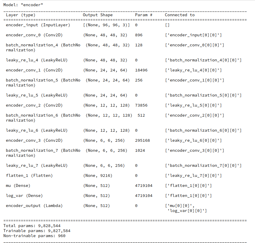
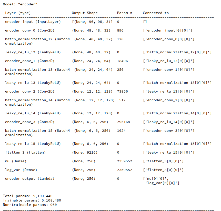
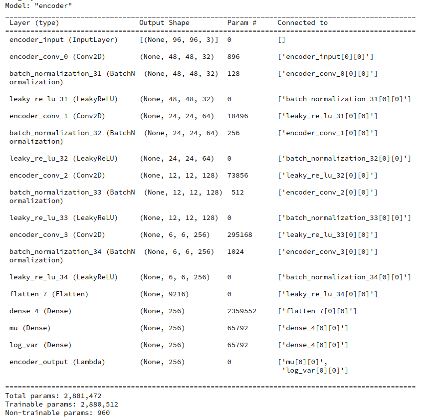
Juypter Cell 8 – Creation of the Encoder model

# Build the Encoder 
# ~~~~~~~~~~~~~~~~~~
MyVae._build_enc()
MyVae.encoder.summary()

Output:

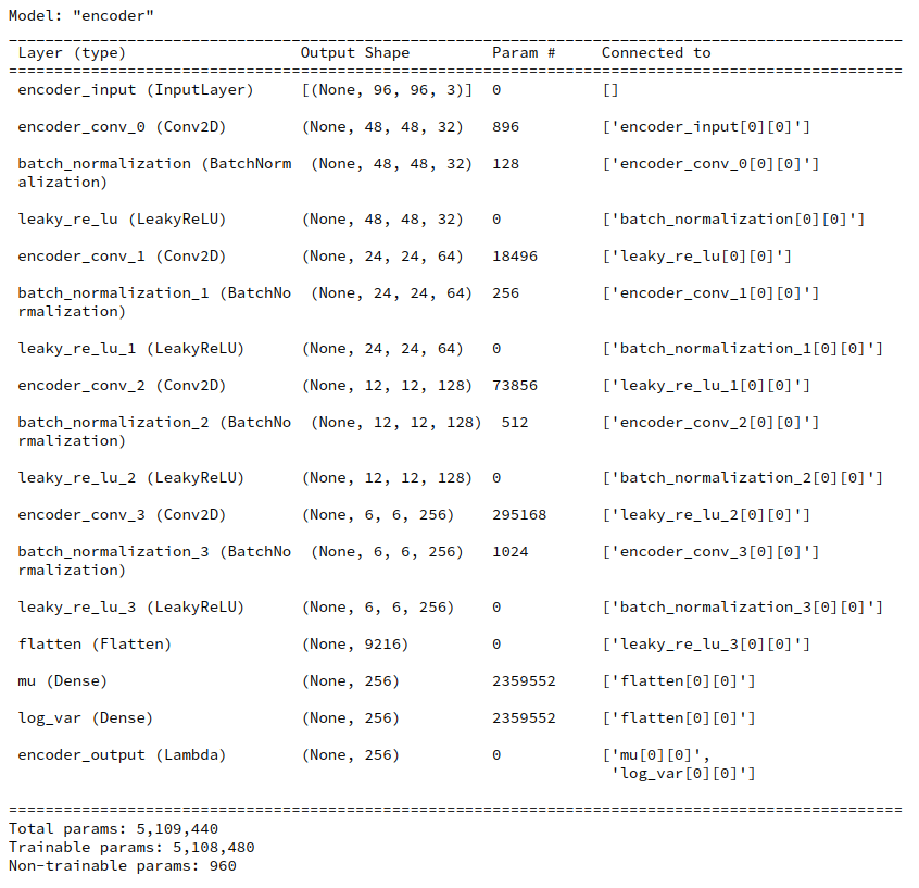
You see that the KL-loss related layers dominate the number of parameters.

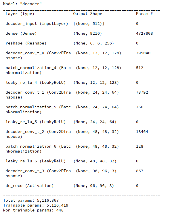
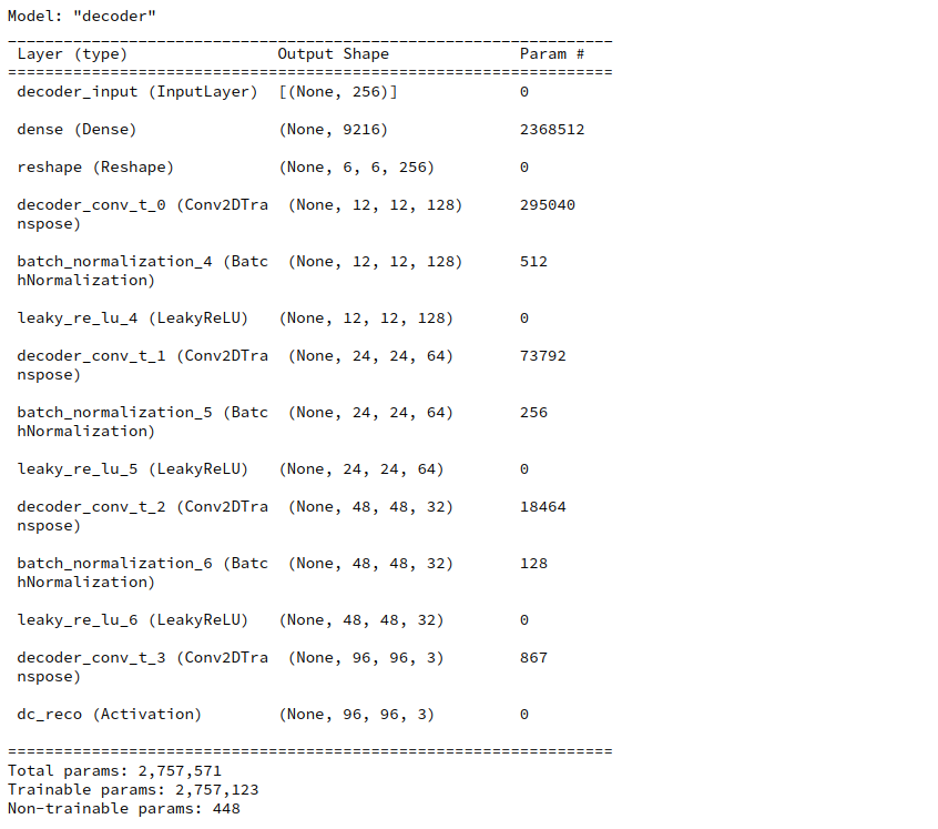
Juypter Cell 9 – Creation of the Decoder model

# Build the Decoder 
# ~~~~~~~~~~~~~~~~~~~
MyVae._build_dec()
MyVae.decoder.summary()

Output:

Building and compiling the full VAE based on GradientTape()

Building and compiling the full VAE based on parameter solution_type = 3 is easy with our class:

Juypter Cell 10 – Creation and compilation of the VAE model

# Build the full AE 
# ~~~~~~~~~~~~~~~~~~~
MyVae._build_VAE()

# Compile the model 
learning_rate = 0.0005
MyVae.compile_myVAE(learning_rate=learning_rate)

Note that internally an instance of class “VAE” is built which handles all loss calculations including the KL-contribution. Compilation and inclusion of an Adam optimizer is also handled internally. Our classes make or life easy …

Our initial learning_rate is relatively small. I followed recommendations of D. Foster’s book on “Generative Deep Learning” regarding this point. A value of 1.e-4 does not change much regarding the number of epochs for convergence.

Due to the chosen low dimension of the latent space the total number of trainable parameters is relatively moderate.

Prepare saving and loading of model parameters

To save some precious computational time (and energy consumption) in the future we need a basic option to save and load model weight parameters. I only describe a direct method; I leave it up to the reader to define a related Callback.

Juypter Cell 11 – Paths to save or load weight parameters

path_model_save_dir = 'YOUR_PATH_TO_A_WEIGHT_SAVING_DIR'

dir_name = 'MyVAE3_sol3_act0_loss0_epo24_fact_5p0emin0_ba128_lay32-64-128-256/'
path_dir = path_model_save_dir + dir_name
if not os.path.isdir(path_dir): 
    os.mkdir(path_dir, mode = 0o755)

dir_all_name = 'all/'
dir_enc_name = 'enc/'
dir_dec_name = 'dec/'

path_dir_all = path_dir + dir_all_name
if not os.path.isdir(path_dir_all): 
    os.mkdir(path_dir_all, mode = 0o755)

path_dir_enc = path_dir + dir_enc_name
if not os.path.isdir(path_dir_enc): 
    os.mkdir(path_dir_enc, mode = 0o755)

path_dir_dec = path_dir + dir_dec_name
if not os.path.isdir(path_dir_dec): 
    os.mkdir(path_dir_dec, mode = 0o755)

name_all = 'all_weights.hd5'
name_enc = 'enc_weights.hd5'
name_dec = 'dec_weights.hd5'

#save all weights
path_all = path_dir + dir_all_name + name_all
path_enc = path_dir + dir_enc_name + name_enc
path_dec = path_dir + dir_dec_name + name_dec

You see that I define separate files in “hd5” format to save parameters of both the full model as well as of its Encoder and Decoder parts.

If we really wanted to load saved weight parameters we could set the parameter “b_load_weight_parameters” in the next cell to “True” and execute the cell code:

Juypter Cell 12 – Load saved weight parameters into the VAE model

b_load_weight_parameters = False

if b_load_weight_parameters:
    MyVae.model.load_weights(path_all)

Training and saving calculated weights

We are ready to perform a training run. For our 170,000 training images and the parameters set I needed a bit more than 18 epochs, namely 24. I did this in two steps – first 18 epochs and then another 6.

Juypter Cell 13 – Load saved weight parameters into the VAE model

INITIAL_EPOCH = 0 

#n_epochs      = 18
n_epochs      = 6

MyVae.set_enc_to_train()
MyVae.train_myVAE(   
             data_flow
            , b_use_generator = True 
            , epochs = n_epochs
            , initial_epoch = INITIAL_EPOCH
            )

The total loss starts in the beginning with a value above 6,900 and quickly closes in to something like 5,100 and below. The KL-loss during raining rises continuously from something like 30 to 176 where it stays almost constant. The 6 epochs after epoch 18 gave the following result:

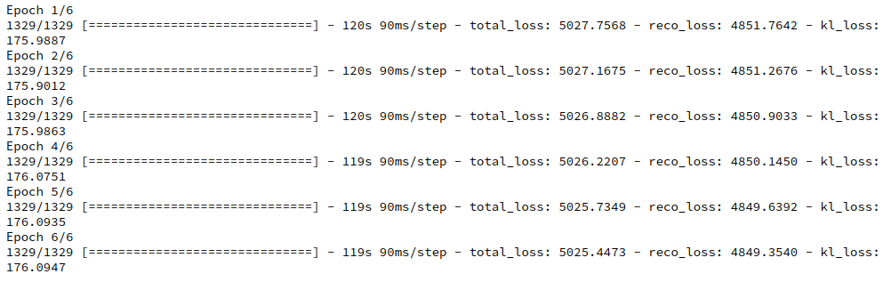
I stopped the calculation at this point – though a full convergence may need some more epochs.

You see that an epoch takes about 2 minutes GPU time (on a GTX960; a modern graphics card will deliver far better values). For 170,000 images the training really costs. On the other side you get a broader variation of face properties in the resulting artificial images later on.

After some epoch we may want to save the weights calculated. The next Jupyter cell shows how.

Juypter Cell 14 – Save weight parameters to disk

print(path_all)
MyVae.model.save_weights(path_all)
print("saving all weights is finished")

print()
#save enc weights
print(path_enc)
MyVae.encoder.save_weights(path_enc)
print("saving enc weights is finished")

print()
#save dec weights
print(path_dec)
MyVae.decoder.save_weights(path_dec)
print("saving dec weights is finished")

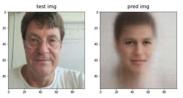
How to test the reconstruction quality?

After training you may first want to test the reconstruction quality of the VAE’s Decoder with respect to training or test images. Unfortunately, I cannot show you original data of the Celeb A dataset. However, the following code cells will help you to do the test by yourself.

Juypter Cell 15 – Choose images and compare them to their reconstructed counterparts

# We choose 14 "random" images from the x_train dataset
# ~~~~~~~~~~~~~~~~~~~~~~~~~~~~~~~~~~~~~~~~~~~~~~~~~~~~
from numpy.random import MT19937
from numpy.random import RandomState, SeedSequence
# For another method to create reproducale "random numbers" see https://albertcthomas.github.io/good-practices-random-number-generators/

n_to_show = 7  # per row 

# To really recover all data we must have one and the same input dataset per training run 
l_seed = [33, 44]   #l_seed = [33, 44, 55, 66, 77, 88, 99]
num_exmpls = len(l_seed)
print(num_exmpls) 

# a list to save the image rows 
l_img_orig_rows = []
l_img_reco_rows = []

start_time = time.perf_counter()

# Set the Encoder to prediction = epsilon * 0.0 
# MyVae.set_enc_to_predict()

for i in range(0, num_exmpls):

    # fixed random distribution 
    rs1 = RandomState(MT19937( SeedSequence(l_seed[i]) ))

    # indices of example array selected from the test images 
    #example_idx = np.random.choice(range(len(x_test)), n_to_show)
    example_idx    = rs1.randint(0, len(x_train), n_to_show)
    example_images = x_train[example_idx]

    # calc points in the latent space 
    if solution_type == 3:
        z_points, mu, logvar  = MyVae.encoder.predict(example_images)
    else:
        z_points  = MyVae.encoder.predict(example_images)

    # Reconstruct the images - note that this results in an array of images  
    reconst_images = MyVae.decoder.predict(z_points)

    # save images in a list 
    l_img_orig_rows.append(example_images)
    l_img_reco_rows.append(reconst_images)

end_time = time.perf_counter()
cpu_time = end_time - start_time

# Reset the Encoder to prediction = epsilon * 1.00 
# MyVae.set_enc_to_train()

print()
print("n_epochs : ", n_epochs, ":: CPU-time to reconstr. imgs: ", cpu_time) 

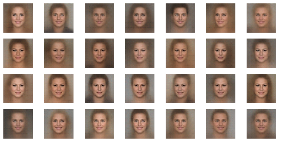
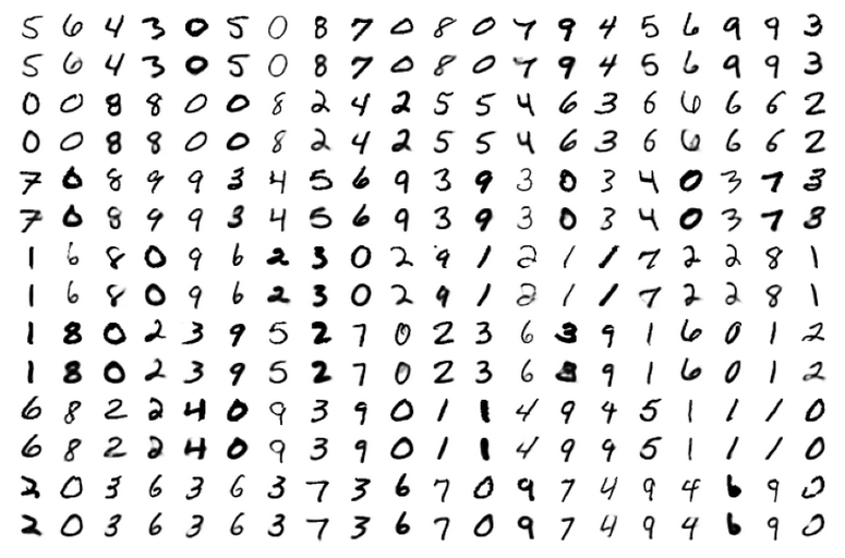
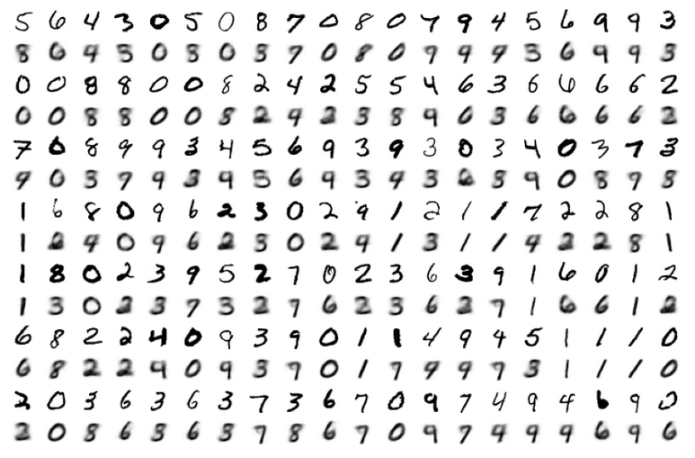
We save the selected original images and the reconstructed images in Python lists.
We then display the original images in one row of a matrix and the reconstructed ones in a row below. We arrange 7 images per row.

Juypter Cell 16 – display original and reconstructed images in a matrix-like array

# Build an image mesh 
# ~~~~~~~~~~~~~~~~~~~~
fig = plt.figure(figsize=(16, 8))
fig.subplots_adjust(hspace=0.2, wspace=0.2)

n_rows = num_exmpls*2 # One more for the original 

for j in range(num_exmpls): 
    offset_orig = n_to_show * j * 2
    for i in range(n_to_show): 
        img = l_img_orig_rows[j][i].squeeze()
        ax = fig.add_subplot(n_rows, n_to_show, offset_orig + i+1)
        ax.axis('off')
        ax.imshow(img, cmap='gray_r')
    
    offset_reco = offset_orig + n_to_show
    for i in range(n_to_show): 
        img = l_img_reco_rows[j][i].squeeze()
        ax = fig.add_subplot(n_rows, n_to_show, offset_reco+i+1)
        ax.axis('off')
        ax.imshow(img, cmap='gray_r')

You will find that the reconstruction quality is rather limited – and not really convincing by any measures regarding details. Only the general shape of faces an their features are reproduced. But, actually, it is this lack of precision regarding details which helps us to create images from arbitrary z-points. I will discuss these points in more detail in a further post.

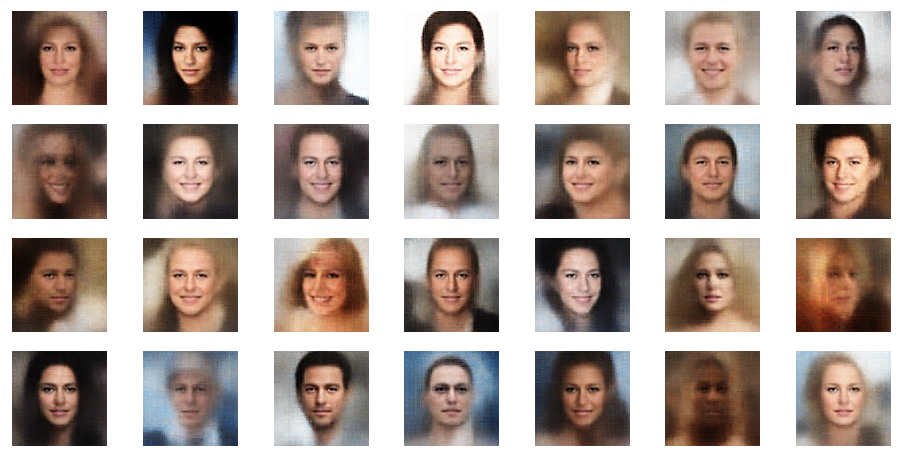
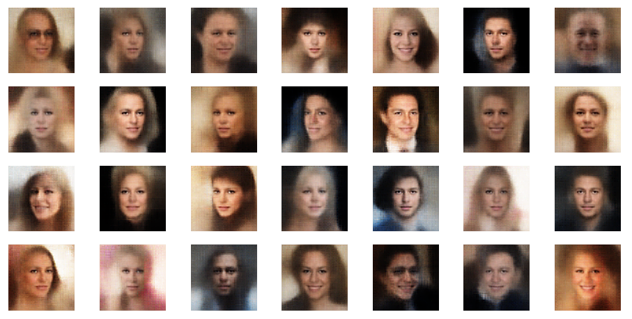
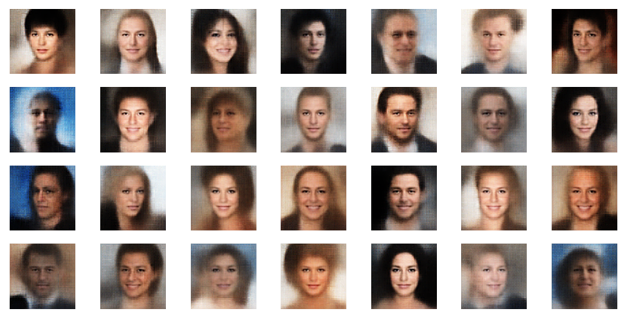
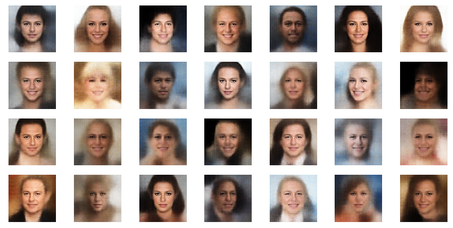
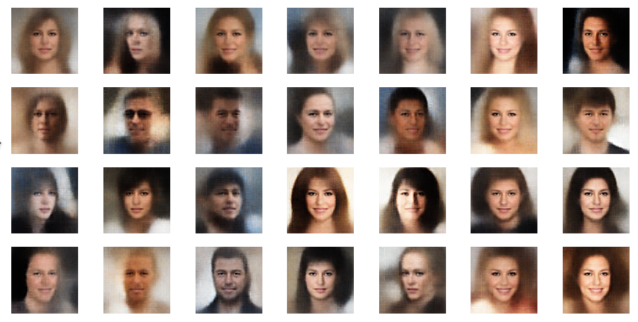
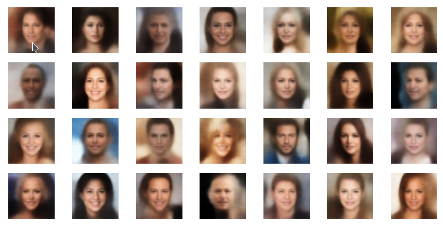
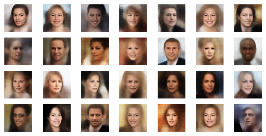
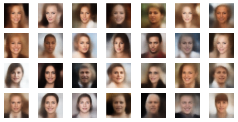
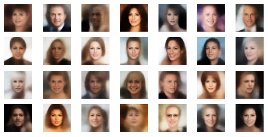
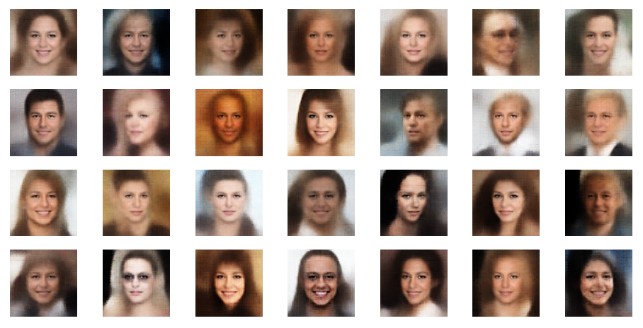
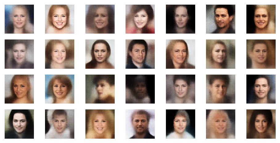
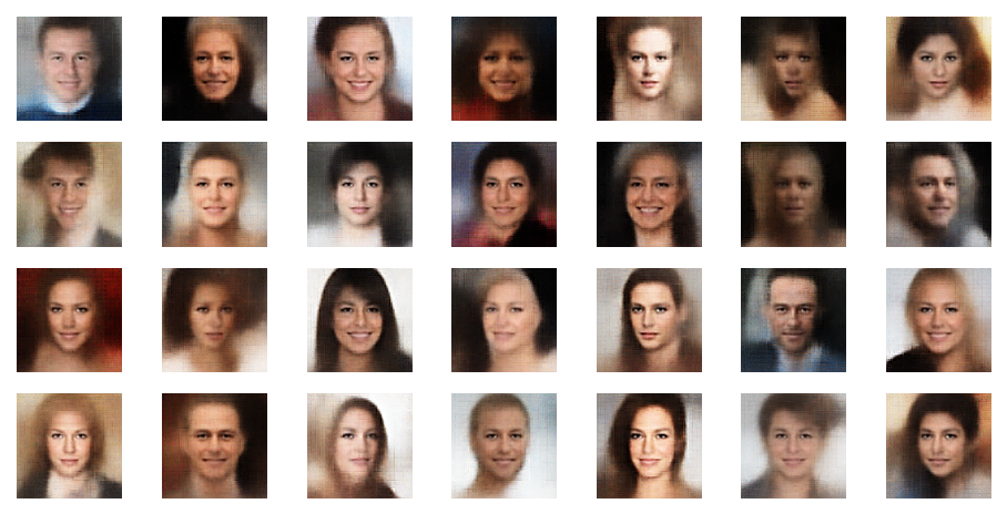
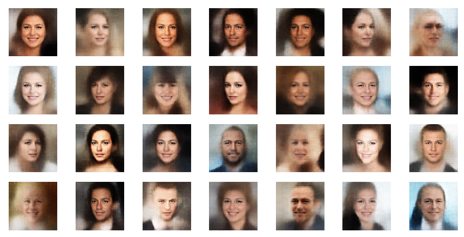
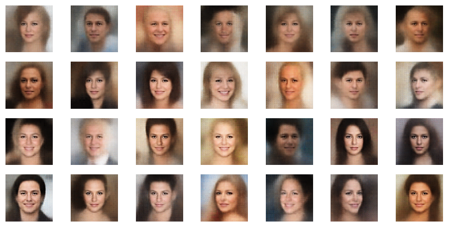
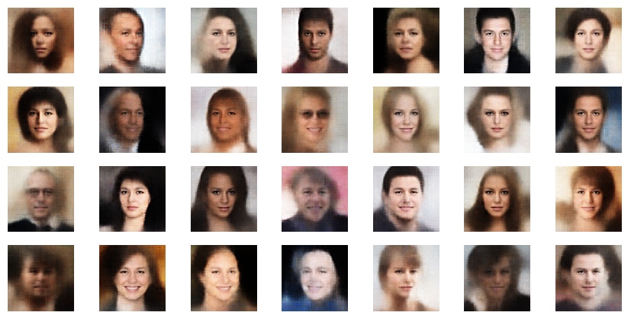
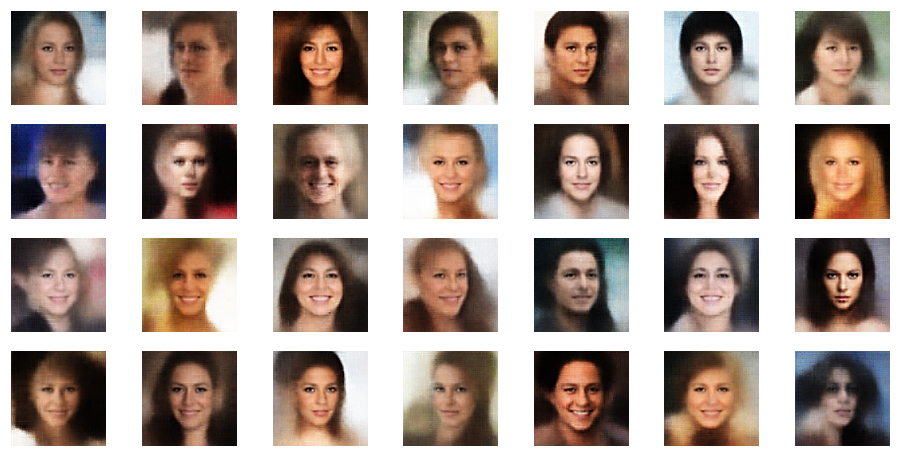
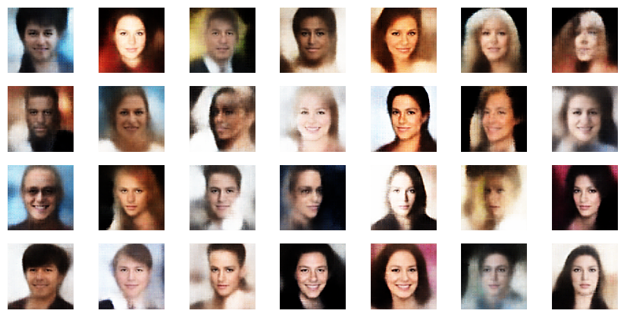
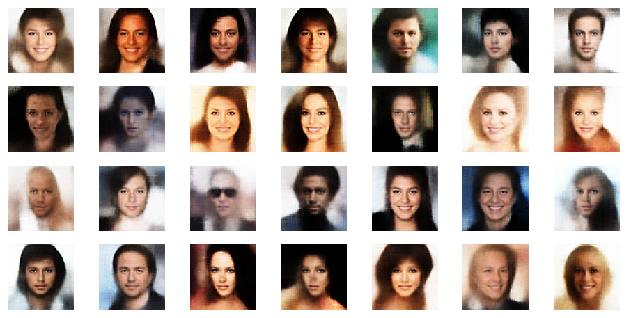
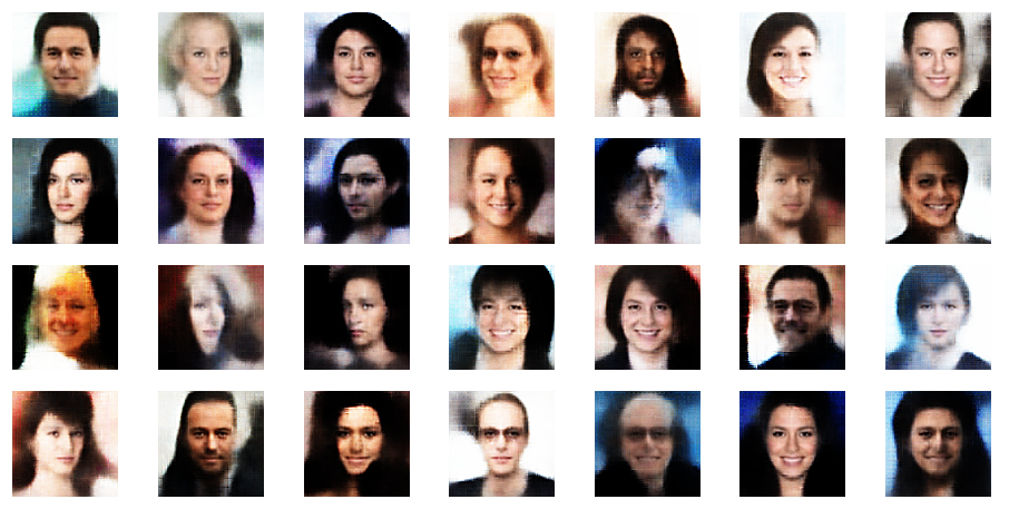
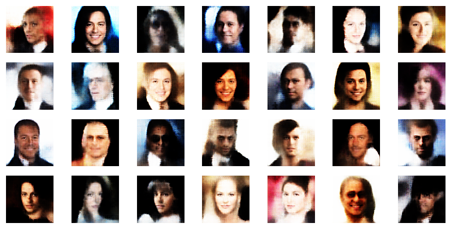
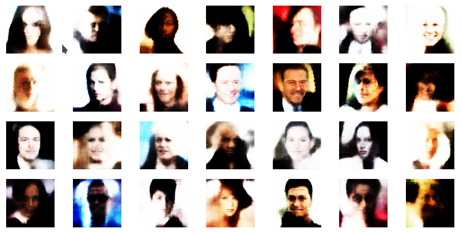
First results: Face images created from randomly distributed points in the latent space

The technique to display images can also be used to display images reconstructed from arbitrary points in the latent space. I will show you various results in another post.

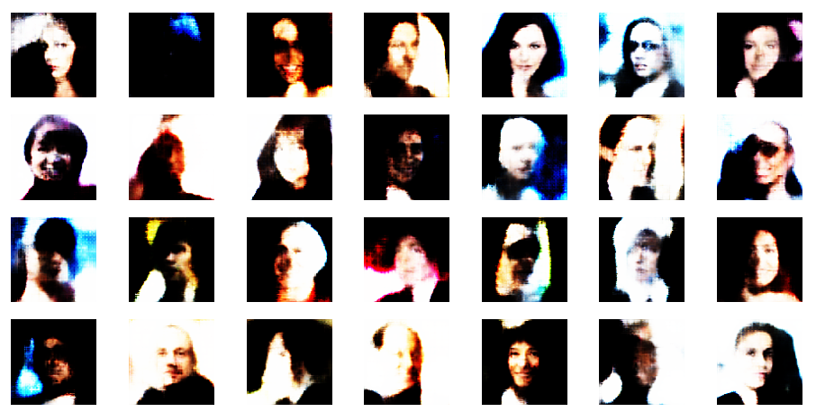
For now just enjoy the creation of images derived from z-points defined by a normal distribution around the center of the latent space:

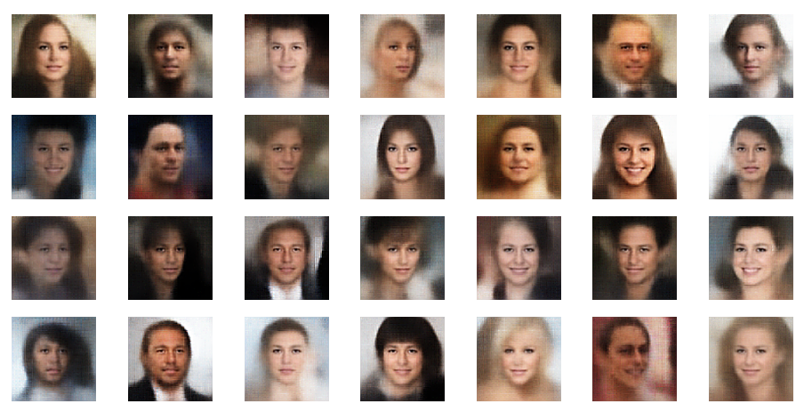
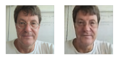
Most of these images look quite convincing and crispy down to details. The sharpness results from some photo-processing with PIL functions after the creation by the VAE. But who said that this is not allowed?

Conclusion

In this post I have presented Jupyter cells with code fragments which may help you to apply the VAE-classes created previously. With the VAE setup discussed above we control the KL-loss by a GradientTape() object.
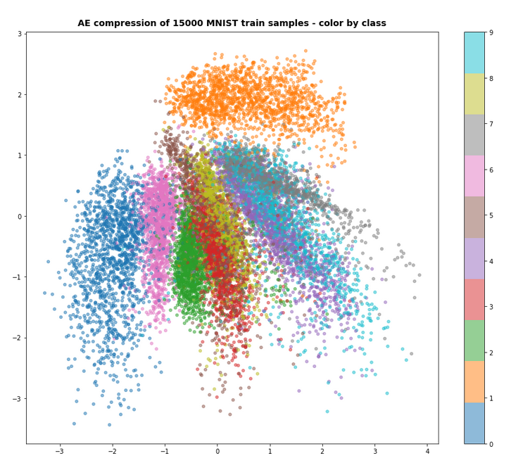
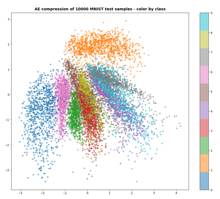
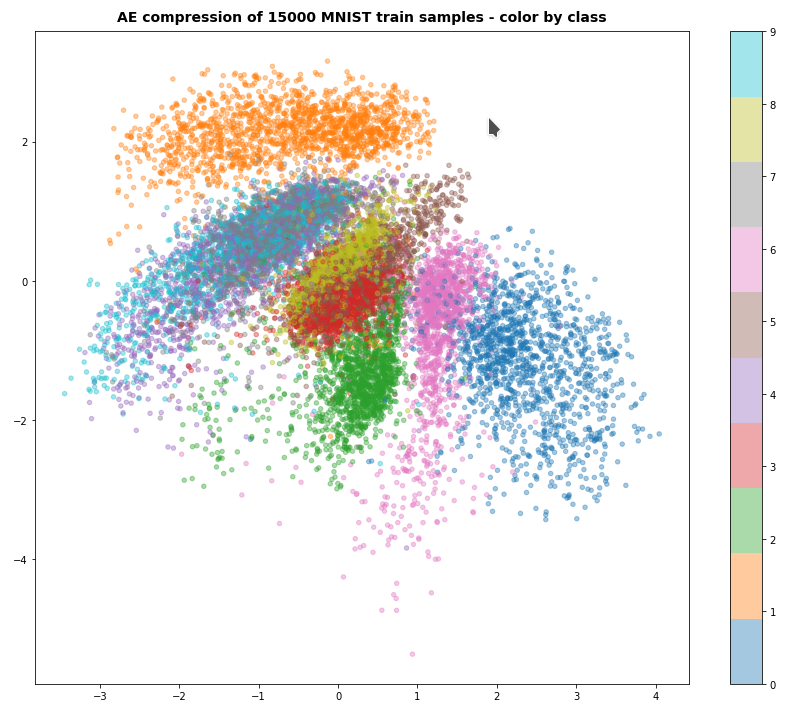
Preliminary results show that the images created of arbitrarily chosen z-points really show heads with human-like faces and hair-dos. In contrast to what a simple AE would produce (see:
Autoencoders, latent space and the curse of high dimensionality – I

In the next post
Variational Autoencoder with Tensorflow – XI – image creation by a VAE trained on CelebA
I will have a look at the distribution of z-points corresponding to the CelebA data and discuss the delicate balance between the representation of details and the generalization of features. With VAEs you cannot get both.

And let us all who praise freedom not forget:
The worst fascist, war criminal and killer living today is the Putler. He must be isolated at all levels, be denazified and sooner than later be imprisoned. Long live a free and democratic Ukraine!


Variational Autoencoder with Tensorflow – VII – KL loss via model.add_loss()

I continue my series on options regarding the treatment of the Kullback-Leibler divergence as a loss [KL loss] in Variational Autoencoder [VAE] setups.

Variational Autoencoder with Tensorflow – I – some basics
Variational Autoencoder with Tensorflow – II – an Autoencoder with binary-crossentropy loss
Variational Autoencoder with Tensorflow – III – problems with the KL loss and eager execution
Variational Autoencoder with Tensorflow – IV – simple rules to avoid problems with eager execution
Variational Autoencoder with Tensorflow – V – a customized Encoder layer for the KL loss
Variational Autoencoder with Tensorflow – VI – KL loss via tensor transfer and multiple output

Our objective is to find solutions which avoid potential problems with the eager execution mode of present Tensorflow 2 implementations. Popular recipes of some teaching books on ML may lead to non-working codes in present TF2 environments. We have already looked at two working alternatives.

In the last post we transferred the “mu” and “log_var” tensors from the Encoder to the Decoder and fed some Keras standard loss functions with these tensors. These functions could in turn be inserted into the model.compile() statement. The approach was a bit complex because it involved multi-input-output model definitions for the Encoder and Decoder.

The present article will discuss a third and lighter approach – namely using the Keras add_loss() mechanism on the level of a Keras model, i.e. model.add_loss().

The advantage of this function is that its parameter interface is not reduced to the form of standardized Keras cost function interfaces which I used in my last post. This gives us flexibility. A solution based on model.add_loss() is also easy to understand and realize on the programming level. It is, however, an approach which may under certain conditions reduce performance by roughly a factor between 1.3 and 1.5 – which is significant. I admit that I have not yet understood what the reasons are. But the concrete solution version I present below works well.

The strategy

The way how to use Keras’ add_loss() functionality is described in the Keras documentation. I quote from this part of TF2’s documentation about the use of add_loss():

This method can also be called directly on a Functional Model during construction. In this case, any loss Tensors passed to this Model must be symbolic and be able to be traced back to the model’s Inputs. These losses become part of the model’s topology and are tracked in get_config.

The documentation also contains a simple example. The strategy is to first define a full VAE model with standard mu and log_var layers in the Encoder part – and afterwards add the KL-loss to this model. This is depicted in the following graphics:

We implement this strategy below via the Python class for a VAE setup which we have used already in the last 4 posts of this series. We control the Keras model setup and the layer construction by the parameter “solution_type”, which I have introduced in my last post.

Cosmetic changes to the Encoder/Decoder parts and the model creation

The class method _build_enc(self, …) can remain as it was defined in the last post. We just have to change the condition for the layer setup as follows:

Change to _build_enc(self, …)

... # see other posts 
...
        # The Encoder Model 
        # ~~~~~~~~~~~~~~~~~~~
        # With extra KL layer or with vae.add_loss()
        if solution_type == 0 or solution_type == 2: 
            self.encoder = Model(self._encoder_input, self._encoder_output)
        
        # Transfer solution => Multiple outputs 
        if solution_type == 1: 
            self.encoder = Model(inputs=self._encoder_input, outputs=[self._encoder_output, self.mu, self.log_var], name="encoder")

Something similar holds for the Decoder part _build_decoder(…):

Change to _build_dec(self, …)

... # see other posts 
...
        # The Decoder model 
        # solution_type == 0/2: Just the decoded input 
        if self.solution_type == 0 or self.solution_type == 2: 
            self.decoder = Model(self._decoder_inp_z, self._decoder_output)
        
        # solution_type == 1: The decoded tensor plus the transferred tensors mu and log_var a for the variational distribution 
        if self.solution_type == 1: 
            self.decoder = Model([self._decoder_inp_z, self._dec_inp_mu, self._dec_inp_var_log], 
                                 [self._decoder_output, self._dec_mu, self._dec_var_log], name="decoder")

A similar change is done regarding the model definition in the method _build_VAE(self):

Change to _build_VAE(self)

        solution_type = self.solution_type
        
        if solution_type == 0 or solution_type == 2:
            model_input  = self._encoder_input
            model_output = self.decoder(self._encoder_output)
            self.model = Model(model_input, model_output, name="vae")

... # see other posts 
...


Changes to the method compile_myVAE(self, learning_rate)

More interesting is a function which we add inside the method compile_myVAE(self, learning_rate, …).

Changes to compile_myVAE(self, learning_rate):

    # Function to compile the full VAE
    # ~~~~~~~~~~~~~~~~~~~~~~~~~~~~~~~~~~~~~~~~~~~~~ 
    def compile_myVAE(self, learning_rate):

        # Optimizer
        # ~~~~~~~~~ 
        optimizer = Adam(learning_rate=learning_rate)
        # save the learning rate for possible intermediate output to files 
        self.learning_rate = learning_rate
        
        # Parameter "fact" will be used by the cost functions defined below to scale the KL loss relative to the BCE loss 
        fact = self.fact
        
        # Function for solution_type == 1
        # ~~~~~~~~~~~~~~~~~~~~~~~~~~~~~~~~~  
        @tf.function
        def mu_loss(y_true, y_pred):
            loss_mux = fact * tf.reduce_mean(tf.square(y_pred))
            return loss_mux
        
        @tf.function
        def logvar_loss(y_true, y_pred):
            loss_varx = -fact * tf.reduce_mean(1 + y_pred - tf.exp(y_pred))    
            return loss_varx

        # Function for solution_type == 2 
        # ~~~~~~~~~~~~~~~~~~~~~~~~~~~~~~~~
        # We follow an approach described at  
        # https://www.tensorflow.org/api_docs/python/tf/keras/layers/Layer
        # NOTE: We can NOT use @tf.function here 
        def get_kl_loss(mu, log_var):
            kl_loss = -fact * tf.reduce_mean(1 + log_var - tf.square(mu) - tf.exp(log_var))
            return kl_loss

        # Required operations for solution_type==2 => model.add_loss()
        # ~~~~~~~~~~~~~~~~~~~~~~~~~~~~~~~~~~~~~~~~~
        res_kl = get_kl_loss(mu=self.mu, log_var=self.log_var)
        if self.solution_type == 2: 
            self.model.add_loss(res_kl)    
            self.model.add_metric(res_kl, name='kl', aggregation='mean')
        
        # Model compilation 
        # ~~~~~~~~~~~~~~~~~~~~
        if self.solution_type == 0 or self.solution_type == 2: 
            self.model.compile(optimizer=optimizer, loss="binary_crossentropy",
                               metrics=[tf.keras.metrics.BinaryCrossentropy(name='bce')])
        
        if self.solution_type == 1: 
            self.model.compile(optimizer=optimizer
                               , loss={'vae_out_main':'binary_crossentropy', 'vae_out_mu':mu_loss, 'vae_out_var':logvar_loss} 
                               #, metrics={'vae_out_main':tf.keras.metrics.BinaryCrossentropy(name='bce'), 'vae_out_mu':mu_loss, 'vae_out_var': logvar_loss }
                               )

I have supplemented function get_kl_loss(mu, log_var). We explicitly provide the tensors “self.mu” and “self.log_var” via the function’s interface and thus follow one of our basic rules for the Keras add_loss()-functionality (see post IV).
Note that this is a MUST to get a working solution for eager execution mode!

Interestingly, the flexibility of model.add_loss() has a price, too. We can NOT use a @tf.function indicator here – in contrast to the standard cost functions which we used in the last post.

Note also that I have added some metrics to get detailed information about the size of the crossentropy-loss and the KL-loss during training!

Cosmetic change to the method for training

Eventually we must include solution_type==2 in method train_myVAE(self, x_train, batch_size, …)

Changes to train_myVAE(self, x_train, batch_size,…)

... # see other posts 
...
        if self.solution_type == 0 or self.solution_type == 2: 
            self.model.fit(     
                x_train
                , x_train
                , batch_size = batch_size
                , shuffle = True
                , epochs = epochs
                , initial_epoch = initial_epoch
            )
        
        if self.solution_type == 1: 
            self.model.fit(     
                x_train
#               Working  
#                , [x_train, t_mu, t_logvar] # we provide some dummy tensors here  
                # by dict: 
                , {'vae_out_main': x_train, 'vae_out_mu': t_mu, 'vae_out_var':t_logvar}
                , batch_size = batch_size
                , shuffle = True
                , epochs = epochs
                , initial_epoch = initial_epoch
                #, verbose=1
                , callbacks=[MyPrinterCallback()]
            )

Some results

We can use a slightly adapted version of the Jupyter notebook cells discussed in post V

Cell 6:

from my_AE_code.models.MyVAE_2 import MyVariationalAutoencoder

z_dim         = 12
solution_type = 2
fact          = 6.5e-4

vae = MyVariationalAutoencoder(
    input_dim = (28,28,1)
    , encoder_conv_filters = [32,64,128]
    , encoder_conv_kernel_size = [3,3,3]
    , encoder_conv_strides = [1,2,2]
    , decoder_conv_t_filters = [64,32,1]
    , decoder_conv_t_kernel_size = [3,3,3]
    , decoder_conv_t_strides = [2,2,1]
    , z_dim = z_dim
    , solution_type = solution_type  
    , act   = 0
    , fact  = fact
)

Cell 11:

BATCH_SIZE = 256
EPOCHS = 37
PRINT_EVERY_N_BATCHES = 100
INITIAL_EPOCH = 0

if solution_type == 2: 
    vae.train_myVAE(     
        x_train[0:60000]
        , batch_size = BATCH_SIZE
        , epochs = EPOCHS
        , initial_epoch = INITIAL_EPOCH
    )

Note that I have changed the BATCH_SIZE to 256 this time; the performance got a bit better then on my old Nvidia 960 GTX:

Epoch 3/37
235/235 [==============================] - 10s 44ms/step - loss: 0.1135 - bce: 0.1091 - kl: 0.0044
Epoch 4/37
235/235 [==============================] - 10s 44ms/step - loss: 0.1114 - bce: 0.1070 - kl: 0.0044
Epoch 5/37
235/235 [==============================] - 10s 44ms/step - loss: 0.1098 - bce: 0.1055 - kl: 0.0044
Epoch 6/37
235/235 [==============================] - 10s 43ms/step - loss: 0.1085 - bce: 0.1041 - kl: 0.0044

This is comparable to data we got for our previous solution approaches. But see an additional section on performance below.

Some results

As in the last posts I show some results for the MNIST data without many comments. The first plot proves the reconstruction abilities of the VAE for a dimension z-dim=12 of the latent space.

MNIST with z-dim=12 and fact=6.5e-4

For z_dim=2 we get a reasonable data point distribution in the latent space due to the KL loss, but the reconstruction ability suffers, of course:

MNIST with z-dim=2 and fact=6.5e-4 – train data distribution in the z-space

For a dimension of z_dim=2 of the latent space and MNIST data we get the following reconstruction chart for data points in a region around the latent space’s origin


A strange performance problem when no class is used

I also tested a version of the approach with model.add_loss() without encapsulating everything in a class. But with the same definition of the Encoder, the Decoder, the model, etc. But all variables as e.g. mu, log_var were directly kept as data of and in the Jupyter notebook. Then a call

n_epochs      = 3
batch_size    = 128
initial_epoch = 0
vae.fit( x_train[0:60000], 
         x_train[0:60000],   # entscheidend ! 
         batch_size=batch_size,
         shuffle=True, 
         epochs = n_epochs, 
         initial_epoch = initial_epoch 
       )

reduced the performance by a factor of 1.5. I have experimented quite a while. But I have no clue at the moment why this happens and how the effect can be avoided. I assume some strange data handling or data transfer between the Jupyter notebook and the graphics card. I can provide details if some developer is interested.

But as one should encapsulate functionality in classes anyway I have not put efforts in a detail analysis.

Conclusion

In this article we have studied an approach to handle the Kullback-Leibler loss via the model.add_loss() functionality of Keras. We supplemented our growing class for a VAE with respective methods. All in all the approach is almost more convenient as the solution based on a special layer and layer.add_loss(); see post V.

However, there seems to exist some strange performance problem when you avoid a reasonable encapsulation in a class and do the modell setup directly in Jupyter cells and for Jupyter variables.

In the next post
Variational Autoencoder with Tensorflow – VIII – TF 2 GradientTape(), KL loss and metrics
I shall have a look at the solution approach recommended by F. Chollet.

Links

We must provide tensors explicitly to model.add_loss()
https://towardsdatascience.com/shared-models-and-custom-losses-in-tensorflow-2-keras-6776ecb3b3a9

 
Ceterum censeo: The worst fascist, war criminal and killer living today, who must be isolated, be denazified and imprisoned, is the Putler. Long live a free and democratic Ukraine!
 

Variational Autoencoder with Tensorflow – V – a customized Encoder layer for the KL loss

I continue with my series on the treatment of the KL loss of Variational Autoencoders in a Keras / TF2.8 environment:

Variational Autoencoder with Tensorflow – I – some basics
Variational Autoencoder with Tensorflow – II – an Autoencoder with binary-crossentropy loss
Variational Autoencoder with Tensorflow – III – problems with the KL loss and eager execution
Variational Autoencoder with Tensorflow – IV – simple rules to avoid problems with eager execution

In the last post it became clear that it might be a good idea to delegate the KL loss calculation to a specific layer within the Encoder model. In this post I discuss the code for such a solution. I am going to encapsulate the construction of a suitable Keras model for the VAE in a class. The class will in further posts be supplemented by more methods for different approaches compatible with TF2.x and eager execution.

The code’s structure has been influenced by the work or books of several people which I want to name explicitly: D. Foster, F. Chollet and Louis Tiao. See the references in the last section of this post.

For the data sets I later want to work with both the Encoder and the Decoder parts of the VAE shall be based upon “convolutional networks” [CNNs] and respective Keras layers. Based on a suggestions of D. Foster and F. Chollet I use a classes interface to provide the parameters of all invoked Conv2D and Conv2DTranspose layers. But in contrast to D. Foster I also indicate how to include different activation functions (e.g. SeLU). In general I also will use the Keras functional API to define and add layers to the VAE model.

Imports to make Keras model and layer classes work

Below I discuss step by step parts of the code I put into a Python module to be used later in Jupyter notebooks. First we need to import some Python modules; note that you may have to add further statements which import personal modules from paths at your local machine:

import sys
import numpy as np
import os

import tensorflow as tf
from tensorflow.keras.layers import Layer, Input, Conv2D, Flatten, Dense, Conv2DTranspose, Reshape, Lambda, \
                                    Activation, BatchNormalization, ReLU, LeakyReLU, ELU, Dropout, AlphaDropout
from tensorflow.keras.models import Model
# to be consistent with my standard loading of the Keras backend in Jupyter notebooks:  
from tensorflow.keras import backend as B      
from tensorflow.keras.optimizers import Adam

A class for a special Encoder layer

Following the ideas discussed in my last post I now add a class which later allows for the setup of a special customized Keras layer in the Encoder model. This layer will calculate the KL loss for us. To be able to do so, the implementation interface “call()” receives a variable “inputs” which contains references to the mu and var_log layers of the Encoder (see the two last posts in this series).

class My_KL_Layer(Layer):
    '''
    @note: Returns the input layers ! Required to allow for z-point calculation
           in a final Lambda layer of the Encoder model    
    '''
    # Standard initialization of layers 
    def __init__(self, *args, **kwargs):
        self.is_placeholder = True
        super(My_KL_Layer, self).__init__(*args, **kwargs)

    # The implementation interface of the Layer
    def call(self, inputs, fact = 4.5e-4):
        mu      = inputs[0]
        log_var = inputs[1]
        # Note: from other analysis we know that the backend applies tf.math.functions 
        # "fact" must be adjusted - for MNIST reasonable values are in the range of 0.65e-4 to 6.5e-4
        kl_mean_batch = - fact * B.mean(1 + log_var - B.square(mu) - B.exp(log_var))
        # We add the loss via the layer's add_loss() - it will be added up to other losses of the model     
        self.add_loss(kl_mean_batch, inputs=inputs)
        # We add the loss information to the metrics displayed during training 
        self.add_metric(kl_mean_batch, name='kl', aggregation='mean')
        return inputs

An important point is that a layer based on this class must return its input, namely the mu and var_log layers, for the z-point calculations in the final Encoder layer.

Note that we do not only add the loss to other losses of an eventual VAE model via the layer’s “add_loss()” method, but that we also ensure to get some information about the the size of the KL loss during training by adding the loss to the metrics.

A general class to setup a VAE build on CNNs for Encoder and Decoder

We now build a class to create the essential parts of a VAE. The class will provide the required flexibility and allow for future extensions comprising other TF2.x compatible solutions for KL loss calculations. (In this post we only use a customized layer to get the KL loss).
We start with the classes “__init__” function, which basically transfers saves parameters into class variables.

# The Main class 
# ~~~~~~~~~~~~~~
class MyVariationalAutoencoder():
    '''
    Coding suggestions of D. Foster and F. Chollet were modified and extended by RMO 
    @version: V0.1, 25.04 
    @change:  added b_build_all 
    @version: V0.2, 08.05 
    @change:  Handling of the KL-loss via functions (partially not working)  
    @version: V0.3, 29.05 
    @change:  Handling of the KL-loss function via a customized Encoder layer 
    '''
    
    def __init__(self
        , input_dim                  # the shape of the input tensors (for MNIST (28,28,1)) 
        , encoder_conv_filters       # number of maps of the different Conv2D layers   
        , encoder_conv_kernel_size   # kernel sizes of the Conv2D layers 
        , encoder_conv_strides       # strides - here also used to reduce spatial resolution avoid pooling layers 
                                     # used instead of Pooling layers 
        , decoder_conv_t_filters     # number of maps in Con2DTranspose layers 
        , decoder_conv_t_kernel_size # kernel sizes of Conv2D Transpose layers  
        , decoder_conv_t_strides     # strides for Conv2dTranspose layers - inverts spatial resolution
        , z_dim                      # A good start is 16 or 24  
        , solution_type  = 0         # Which type of solution for the KL loss calculation ?
        , act            = 0         # Which type of activation function?  
        , fact           = 0.65e-4   # Factor for the KL loss (0.5e-4 < fact < 1.e-3is reasonable)    
        , use_batch_norm = False     # Shall BatchNormalization be used after Conv2D layers? 
        , use_dropout    = False     # Shall statistical dropout layers be used for tregularization purposes ? 
        , b_build_all    = False  # Added by RMO - full Model is build in 2 steps 
        ):
        
        '''
        Input: 
        The encoder_... and decoder_.... variables are Python lists,
        whose length defines the number of Conv2D and Conv2DTranspose layers 
        
        input_dim : Shape/dimensions of the input tensor - for MNIST (28,28,1) 
        encoder_conv_filters:     List with the number of maps/filters per Conv2D layer    
        encoder_conv_kernel_size: List with the kernel sizes for the Conv-Layers   
        encoder_conv_strides:     List with the strides used for the Conv-Layers   

        act :  determines activation function to use (0: LeakyRELU, 1:RELU , 2: SELU)
               !!!! NOTE: !!!!
               If SELU is used then the weight kernel initialization and the dropout layer need to be special   
               https://github.com/christianversloot/machine-learning-articles/blob/main/using-selu-with-tensorflow-and-keras.md
               AlphaDropout instead of Dropout + LeCunNormal for kernel initializer
        z_dim : dimension of the "latent_space"
        solution_type : Type of solution for KL loss calculation (0: Customized Encoder layer, 
                                                                  1: model.add_loss()
                                                                  2: definition of training step with Gradient.Tape()
        
        use_batch_norm = False   # True : We use BatchNormalization   
        use_dropout    = False   # True : We use dropout layers (rate = 0.25, see Encoder)
        b_build_all    = False   # True : Full VAE Model is build in 1 step; 
                                   False: Encoder, Decoder, VAE are build in separate steps   
        '''
        
        self.name = 'variational_autoencoder'

        # Parameters for Layers which define the Encoder and Decoder 
        self.input_dim                  = input_dim
        self.encoder_conv_filters       = encoder_conv_filters
        self.encoder_conv_kernel_size   = encoder_conv_kernel_size
        self.encoder_conv_strides       = encoder_conv_strides
        self.decoder_conv_t_filters     = decoder_conv_t_filters
        self.decoder_conv_t_kernel_size = decoder_conv_t_kernel_size
        self.decoder_conv_t_strides     = decoder_conv_t_strides
        
        self.z_dim = z_dim

        # Check param for activation function 
        if act < 0 or act > 2: 
            print("Range error: Parameter " + str(act) + " has unknown value ")  
            sys.exit()
        else:
            self.act = act 
        
        # Factor to scale the KL loss relative to the Binary Cross Entropy loss 
        self.fact = fact 
        
        # Check param for solution approach  
        if solution_type < 0 or solution_type > 2: 
            print("Range error: Parameter " + str(solution_type) + " has unknown value ")  
            sys.exit()
        else:
            self.solution_type = solution_type 

        self.use_batch_norm = use_batch_norm
        self.use_dropout    = use_dropout

        # Preparation of some variables to be filled later 
        self._encoder_input  = None  # receives the Keras object for the Input Layer of the Encoder 
        self._encoder_output = None  # receives the Keras object for the Output Layer of the Encoder 
        self.shape_before_flattening = None # info of the Encoder => is used by Decoder 
        self._decoder_input  = None  # receives the Keras object for the Input Layer of the Decoder
        self._decoder_output = None  # receives the Keras object for the Output Layer of the Decoder

        # Layers / tensors for KL loss 
        self.mu      = None # receives special Dense Layer's tensor for KL-loss 
        self.log_var = None # receives special Dense Layer's tensor for KL-loss 

        # Parameters for SELU - just in case we may need to use it somewhere 
        # https://keras.io/api/layers/activations/ see selu
        self.selu_scale = 1.05070098
        self.selu_alpha = 1.67326324

        # The number of Conv2D and Conv2DTranspose layers for the Encoder / Decoder 
        self.n_layers_encoder = len(encoder_conv_filters)
        self.n_layers_decoder = len(decoder_conv_t_filters)

        self.num_epoch = 0 # Intialization of the number of epochs 

        # A matrix for the values of the losses 
        self.std_loss  = tf.TensorArray(tf.float32, size=0, dynamic_size=True, clear_after_read=False)

        # We only build the whole AE-model if requested
        self.b_build_all = b_build_all
        if b_build_all:
            self._build_all()

Note that for the present post we (can) only use “solution_type = 0” !

A method to build the Encoder

The class shall provide a method to build the Encoder. For our present purposes including a customized layer based on the class “My_KL_Layer”. This layer just returns its input – namely the layers “mu” and “var_log” for the variational calculation of z-points, but it also calculates the KL loss which is added to other model losses.

    # Method to build the Encoder
    # ~~~~~~~~~~~~~~~~~~~~~~~~~~~ 
    def _build_enc(self, solution_type = 0, fact=-1.0):
        '''
        Encoder 
        @summary: Method to build the Encoder part of the AE 
                  This will be a CNN defined by the parameters to __init__   
         
        @note:    For self.solution = 0, we add an extra layer to calculate the KL loss 
        @note:    The last layer uses a sigmoid activation to create the output 
                  This may not be compatible with some scalers applied to the input data (images)    
        '''       

        # Check whether "fact" for the KL loss shall be overwritten
        if fact < 0:
            fact = self.fact  
        
        # Preparation: We later need a function to calculate the z-points in the latent space 
        # this function will be used by an eventual Lambda layer of the Encoder 
        def z_point_sampling(args):
            '''
            A point in the latent space is calculated statistically 
            around an optimized mu for each sample 
            '''
            mu, log_var = args # Note: These are 1D tensors !
            epsilon = B.random_normal(shape=B.shape(mu), mean=0., stddev=1.)
            return mu + B.exp(log_var / 2) * epsilon

        
        # Input "layer"
        self._encoder_input = Input(shape=self.input_dim, name='encoder_input')

        # Initialization of a running variable x for individual layers 
        x = self._encoder_input

        # Build the CNN-part with Conv2D layers 
        # Note that stride>=2 reduces spatial resolution without the help of pooling layers 
        for i in range(self.n_layers_encoder):
            conv_layer = Conv2D(
                filters = self.encoder_conv_filters[i]
                , kernel_size = self.encoder_conv_kernel_size[i]
                , strides = self.encoder_conv_strides[i]
                , padding = 'same'  # Important ! Controls the shape of the layer tensors.    
                , name = 'encoder_conv_' + str(i)
                )
            x = conv_layer(x)
            
            # The "normalization" should be done ahead of the "activation" 
            if self.use_batch_norm:
                x = BatchNormalization()(x)

            # Selection of activation function (out of 3)      
            if self.act == 0:
                x = LeakyReLU()(x)
            elif self.act == 1:
                x = ReLU()(x)
            elif self.act == 2: 
                # RMO: Just use the Activation layer to use SELU with predefined (!) parameters 
                x = Activation('selu')(x) 

            # Fulfill some SELU requirements 
            if self.use_dropout:
                if self.act == 2: 
                    x = AlphaDropout(rate = 0.25)(x)
                else:
                    x = Dropout(rate = 0.25)(x)

        # Last multi-dim tensor shape - is later needed by the decoder 
        self._shape_before_flattening = B.int_shape(x)[1:]

        # Flattened layer before calculating VAE-output (z-points) via 2 special layers 
        x = Flatten()(x)
        
        # "Variational" part - create 2 Dense layers for a statistical distribution of z-points  
        self.mu      = Dense(self.z_dim, name='mu')(x)
        self.log_var = Dense(self.z_dim, name='log_var')(x)

        if solution_type == 0: 
            # Customized layer for the calculation of the KL loss based on mu, var_log data
            # We use a customized layer accoding to a class definition  
            self.mu, self.log_var = My_KL_Layer()([self.mu, self.log_var], fact=fact)
 
        # Layer to provide a z_point in the Latent Space for each sample of the batch 
        self._encoder_output = Lambda(z_point_sampling, name='encoder_output')([self.mu, self.log_var])

        # The Encoder Model 
        self.encoder = Model(self._encoder_input, self._encoder_output)

A method to build the Decoder

The following function should be self-evident; it reverses the Encoder’s operations and uses z-points of the latent space as input.

    # Method to build the Decoder
    # ~~~~~~~~~~~~~~~~~~~~~~~~~~~ 
    def _build_dec(self):
        '''
        Decoder 
        @summary: Method to build the Decoder part of the AE 
                  Normally this will be a reverse CNN defined by the parameters to __init__   
        '''       

        # Input layer - aligned to the shape of the output layer 
        self._decoder_input = Input(shape=(self.z_dim,), name='decoder_input')

        # Here we use the tensor shape info from the Encoder          
        x = Dense(np.prod(self._shape_before_flattening))(self._decoder_input)
        x = Reshape(self._shape_before_flattening)(x)

        # The inverse CNN
        for i in range(self.n_layers_decoder):
            conv_t_layer = Conv2DTranspose(
                filters = self.decoder_conv_t_filters[i]
                , kernel_size = self.decoder_conv_t_kernel_size[i]
                , strides = self.decoder_conv_t_strides[i]
                , padding = 'same' # Important ! Controls the shape of tensors during reconstruction
                                   # we want an image with the same resolution as the original input 
                , name = 'decoder_conv_t_' + str(i)
                )
            x = conv_t_layer(x)

            # Normalization and Activation 
            if i < self.n_layers_decoder - 1:
                # Also in the decoder: normalization before activation  
                if self.use_batch_norm:
                    x = BatchNormalization()(x)
                
                # Choice of activation function
                if self.act == 0:
                    x = LeakyReLU()(x)
                elif self.act == 1:
                    x = ReLU()(x)
                elif self.act == 2: 
                    #x = self.selu_scale * ELU(alpha=self.selu_alpha)(x)
                    x = Activation('selu')(x)
                
                # Adaptions to SELU requirements 
                if self.use_dropout:
                    if self.act == 2: 
                        x = AlphaDropout(rate = 0.25)(x)
                    else:
                        x = Dropout(rate = 0.25)(x)
                
            # Last layer => Sigmoid output 
            # => This requires scaled input => Division of pixel values by 255
            else:
                x = Activation('sigmoid')(x)

        # Output tensor => a scaled image 
        self._decoder_output = x

        # The Decoder model 
        self.decoder = Model(self._decoder_input, self._decoder_output)

Note that we do not include any loss calculations in the Decoder model. The main loss – namely according to the “binary cross entropy” will later be added to the “fit()” method of the full Keras based VAE model.

The full VAE model

We have already created two Keras models for the Encoder and Decoder. We now combine them to the full VAE model and save this model in a variable of the object derived from our class.

    # Function to build the full AE
    # ~~~~~~~~~~~~~~~~~~~~~~~~~~~~~
    def _build_VAE(self):     
        model_input  = self._encoder_input
        model_output = self.decoder(self._encoder_output)
        self.model = Model(model_input, model_output, name="vae")

    # Function to build full AE in one step if requested
    # ~~~~~~~~~~~~~~~~~~~~~~~~~~~~~~~~~~~~~~~~~~~~~~~~~~
    def _build_all(self):
        self._build_enc()
        self._build_dec()
        self._build_VAE()

Compilation

For our present solution with the customized layer for the KL loss we now provide a matching “compile()” function:

    # Function to compile VA-model with a KL-layer in the Encoder 
    # ~~~~~~~~~~~~~~~~~~~~~~~~~~~~~~~~~~~~~~~~~~~~~~~~~~~~~~~~~
    def compile_for_KL_Layer(self, learning_rate):
        if self.solution_type != 0: 
            print("The compile_L() function is only compatible with solution_type = 0")
            sys.exit()
        self.learning_rate = learning_rate
        # Optimizer 
        optimizer = Adam(learning_rate=learning_rate)
        self.model.compile(optimizer=optimizer, loss="binary_crossentropy",
                           metrics=[tf.keras.metrics.BinaryCrossentropy(name='bce')])

This is the place where we include the main contribution to the loss – namely by a “binary cross-entropy” calculation with respect to the differences between the original input tensor top our model and its output tensor. We had to use the function BinaryCrossentropy(name=’bce’) to be able to give the respective output during training a short name. All in all we expect an output during training comprising:

  • the total loss
  • the contribution from the binary_crossentropy
  • the KL contribution

A method for training

We are almost finished. We just need a matching method for starting the training via calling the “fit()“-function of our Keras based VAE model:

    def train_model_with_KL_Layer(self, x_train, batch_size, epochs, initial_epoch = 0):
        self.model.fit(     
            x_train
            , x_train
            , batch_size = batch_size
            , shuffle = True
            , epochs = epochs
            , initial_epoch = initial_epoch
        )

Note that we called the same “x_train” batch of samples twice: The standard “y” output “labels” actually are the input samples (which is, of course, the core characteristic of AEs). We shuffle data during training.

Why use a special function of the class at all and not directly call fit() from Jupyter notebook cells?
Well, at this point we could include multiple other things as custom callbacks (e.g. for special output or model saving) and a scheduler. See e.g. the code of D. Foster at his Github site for variants. For the sake of briefness I skip these techniques in my post.

Jupyter cells to use our class

Let us see how we can use our carefully crafted class with a Jupyter notebook. As I personally gather Python modules (via Eclipse PyDev) in some special folders, I first have to add a path:

Cell 1:

import sys
# !!! ADAPT to YOUR needs !!!!! 
sys.path.append("/projects/GIT/ml_4/")
print(sys.path)

Of course, you must adapt this path to your personal situation.

The next cell contains module imports
Cell 2

import numpy as np
import time 
import os
import sklearn # could be used for scalers
import matplotlib as mpl
from matplotlib import pyplot as plt
from matplotlib.colors import ListedColormap
import matplotlib.patches as mpat 

# tensorflow and keras 
import tensorflow as tf
from tensorflow import keras as K
from tensorflow.python.keras import backend as B 
from tensorflow.keras import models
from tensorflow.keras import layers
from tensorflow.keras import regularizers
from tensorflow.keras import optimizers
from tensorflow.keras import metrics
from tensorflow.keras.datasets import mnist
from tensorflow.keras.optimizers import schedules
from tensorflow.keras.utils import to_categorical
from tensorflow.python.client import device_lib
from tensorflow.keras.datasets import mnist

# My VAE-class 
from my_AE_code.models.My_VAE import MyVariationalAutoencoder

I then suppress some warnings regarding my Nvidia card and list the available Cuda devices.

Cell 3


# Suppress some TF2 warnings on negative NUMA node number
# see https://www.programmerall.com/article/89182120793/
os.environ['TF_CPP_MIN_LOG_LEVEL'] = '3'  # or any {'0', '1', '2'}
tf.config.experimental.list_physical_devices()

We then control resource usage:
Cell 4

# Restrict to GPU and activate jit to accelerate 
# IMPORTANT NOTE: To change any of the following values you MUT restart the notebook kernel ! 
b_tf_CPU_only      = False   # we want to work on a GPU  
tf_limit_CPU_cores = 4 
tf_limit_GPU_RAM   = 2048

if b_tf_CPU_only: 
    tf.config.set_visible_devices([], 'GPU')   # No GPU, only CPU 
    # Restrict number of CPU cores
    tf.config.threading.set_intra_op_parallelism_threads(tf_limit_CPU_cores)
    tf.config.threading.set_inter_op_parallelism_threads(tf_limit_CPU_cores)
else: 
    gpus = tf.config.experimental.list_physical_devices('GPU')
    tf.config.experimental.set_virtual_device_configuration(gpus[0], 
    [tf.config.experimental.VirtualDeviceConfiguration(memory_limit = tf_limit_GPU_RAM)])

# JiT optimizer 
tf.config.optimizer.set_jit(True)

Let us load MNIST for test purposes:
Cell 5

def load_mnist():
    (x_train, y_train), (x_test, y_test) = mnist.load_data()

    x_train = x_train.astype('float32') / 255.
    x_train = x_train.reshape(x_train.shape + (1,))
    x_test = x_test.astype('float32') / 255.
    x_test = x_test.reshape(x_test.shape + (1,))

    return (x_train, y_train), (x_test, y_test)

(x_train, y_train), (x_test, y_test) = load_mnist()

Provide the VAE setup variables to our class:
Cell 6

z_dim = 2
vae = MyVariationalAutoencoder(
    input_dim = (28,28,1)
    , encoder_conv_filters = [32,64,128]
    , encoder_conv_kernel_size = [3,3,3]
    , encoder_conv_strides = [1,2,2]
    , decoder_conv_t_filters = [64,32,1]
    , decoder_conv_t_kernel_size = [3,3,3]
    , decoder_conv_t_strides = [2,2,1]
    , z_dim = z_dim
    , act   = 0
    , fact  = 5.e-4
)

Set up the Encoder:
Cell 7

# overwrite the KL fact from the class 
fact = 2.e-4 
vae._build_enc(fact=fact)
vae.encoder.summary()

Build the Decoder:
Cell 8

vae._build_dec()
vae.decoder.summary()

Build the VAE model:
Cell 9

vae._build_VAE()
vae.model.summary()

Compile
Cell 10

LEARNING_RATE = 0.0005
vae.compile_for_KL_Layer(LEARNING_RATE)

Train / fit the model to the training data
Cell 11

BATCH_SIZE = 128
EPOCHS = 6     # for real runs ca. 40 
INITIAL_EPOCH = 0
vae.train_model_with_KL_Layer(     
    x_train[0:60000]
    , batch_size = BATCH_SIZE
    , epochs = EPOCHS
    , initial_epoch = INITIAL_EPOCH
)

For the given parameters I got the following output on my old GTX960

Epoch 1/6
469/469 [==============================] - 12s 24ms/step - loss: 0.2613 - bce: 0.2589 - kl: 0.0024
Epoch 2/6
469/469 [==============================] - 12s 25ms/step - loss: 0.2174 - bce: 0.2159 - kl: 0.0015
Epoch 3/6
469/469 [==============================] - 11s 23ms/step - loss: 0.2100 - bce: 0.2085 - kl: 0.0015
Epoch 4/6
469/469 [==============================] - 11s 23ms/step - loss: 0.2057 - bce: 0.2042 - kl: 0.0015
Epoch 5/6
469/469 [==============================] - 11s 23ms/step - loss: 0.2034 - bce: 0.2019 - kl: 0.0015
Epoch 6/6
469/469 [==============================] - 11s 23ms/step - loss: 0.2019 - bce: 0.2004 - kl: 0.0015

So 11 secs for an epoch of 60,000 samples with batch-size = 128 is a reference point. Note that this is obviously faster than what we got for the solution discussed in the last post.

Just to give you an impression of other results:
For z_dim = 2, fact = 2.e-4 and 60 epochs I got something like the following data point distribution in the latent space:

I shall discuss more results – also for other test data sets – in future posts in this blog.

Conclusion

In this post we have build a class to set up a VAE based on an Encoder and a Decoder model with Conv2D and Conv2dTranspose layers. We delegated the calculation of the KL loss to a customized layer of the Encoder, whilst the main loss contribution was defined in form of a binary-crossentropy evaluation with the help of the fit()-function of the VAE model. All loss contributions were displayed as “metrics” elements during training. The presented solution is fully compatible with Tensorflow 2.8 and eager execution. It is in my opinion also elegant and very Keras oriented as all important operations are encapsulated in a continuous sequence of layers. We also found this to be a relatively fast solution.

In the next post of this series
Variational Autoencoder with Tensorflow – VI – KL loss via tensor transfer and multiple output
we are going to use our class to adapt an older suggestion of D.Foster to the requirements of TF2.8.

References

F. Chollet, Deep Learning mit Python und Keras, 2018, 1-te dt. Auflage, mitp Verlags GmbH & Co.KG, Frechen

D. Foster, “Generatives Deep Learning”, 2020, 1-te dt. Auflage, dpunkt Verlag, Heidelberg in Kooperation mit Media Inc.O’Reilly, ISBN 978-3-960009-128-8. See Kap. 3 and the VAE code published at
https://github.com/davidADSP/GDL_code/

Louis Tiao, “Implementing Variational Autoencoders in Keras: Beyond the Quickstart Tutorial”, 2017, http://louistiao.me/posts/implementing-variational-autoencoders-in-keras-beyond-the-quickstart-tutorial/

Recommendation: The article of L. Tiao is not only interesting regarding Keras modularity. I like it very much also for his mathematical depth. I highly recommend his article as a source of inspiration, especially with respect to alternative divergences. Please, also follow Tiao’s list of well selected literature references.

And before I forget it:
Ceterum censeo: The worst living fascist and war criminal today, who must be isolated, denazified and imprisoned, is the Putler.