Welcome back to my readers who followed me through the (painful?) process of writing a Python class to simulate a “Multilayer Perceptron” [MLP]. The pain in my case resulted from the fact that I am still a beginner in Machine Learning [ML] and Python. Nevertheless, I hope that we have meanwhile acquired some basic understanding of how a MLP works and “learns”. During the course of the last articles we had a close look at such nice things as “forward propagation”, “gradient descent”, “mini-batches” and “error backward propagation”. For the latter I gave you a mathematical description to grasp the background of the matrix operations involved.
Where do we stand after 10 articles and a PDF on the math?
A simple program for an ANN to cover the Mnist dataset – X – mini-batch-shuffling and some more tests
A simple program for an ANN to cover the Mnist dataset – IX – First Tests
A simple program for an ANN to cover the Mnist dataset – VIII – coding Error Backward Propagation
A simple program for an ANN to cover the Mnist dataset – VII – EBP related topics and obstacles
A simple program for an ANN to cover the Mnist dataset – VI – the math behind the „error back-propagation“
A simple program for an ANN to cover the Mnist dataset – V – coding the loss function
A simple program for an ANN to cover the Mnist dataset – IV – the concept of a cost or loss function
A simple program for an ANN to cover the Mnist dataset – III – forward propagation
A simple program for an ANN to cover the Mnist dataset – II – initial random weight values
A simple program for an ANN to cover the Mnist dataset – I – a starting point
We have a working code
- with some parameters to control layers and node numbers, learning and momentum rates and regularization,
- with many dummy parts for other output and activation functions than the sigmoid function we used so far,
- with prepared code fragments for applying MSE instead of “Log Loss” as a cost function,
- and with dummy parts for handling different input datasets than the MNIST example.
The code is not yet optimized; it includes e.g. many statements for tests which we should eliminate or comment out. A completely open conceptual aspect is the optimization of the adaption of the learning rate; it is very primitive so far. We also need an export/import functionality to be able to perform training with a series of limited epoch numbers per run.
We also should save the weights and accuracy data after a fixed epoch interval to be able to analyze a bit more after training. Another idea – though probably costly – is to even perform intermediate runs on the test data set an get some information on the development of the averaged error on the test data set.
Despite all these deficits, which we need to cover in some more articles, we are already able to perform an insightful task – namely to find out with which numbers and corresponding images of the MNIST data set our MLP has problems with. This leads us to the topics of a confusion matrix and other measures for the accuracy of our algorithm.
However, before we look at these topics, we first create some useful code, which we can save inside cells of the Jupyter notebook we maintain for testing our class “MyANN”.
Some functions to evaluate the prediction capability of our ANN after training
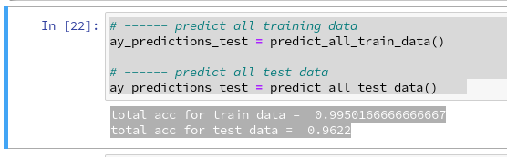
For further analysis we shall apply the following functions later on:
# ------ predict results for all test data
# *************************
def predict_all_test_data():
size_set = ANN._X_test.shape[0]
li_Z_in_layer_test = [None] * ANN._n_total_layers
li_Z_in_layer_test[0] = ANN._X_test
# Transpose input data matrix
ay_Z_in_0T = li_Z_in_layer_test[0].T
li_Z_in_layer_test[0] = ay_Z_in_0T
li_A_out_layer_test = [None] * ANN._n_total_layers
# prediction by forward propagation of the whole test set
ANN._fw_propagation(li_Z_in = li_Z_in_layer_test, li_A_out = li_A_out_layer_test, b_print = False)
ay_predictions_test = np.argmax(li_A_out_layer_test[ANN._n_total_layers-1], axis=0)
# accuracy
ay_errors_test = ANN._y_test - ay_predictions_test
acc = (np.sum(ay_errors_test == 0)) / size_set
print ("total acc for test data = ", acc)
def predict_all_train_data():
size_set = ANN._X_train.shape[0]
li_Z_in_layer_test = [None] * ANN._n_total_layers
li_Z_in_layer_test[0] = ANN._X_train
# Transpose
ay_Z_in_0T = li_Z_in_layer_test[0].T
li_Z_in_layer_test[0] = ay_Z_in_0T
li_A_out_layer_test = [None] * ANN._n_total_layers
ANN._fw_propagation(li_Z_in = li_Z_in_layer_test, li_A_out = li_A_out_layer_test, b_print = False)
Result = np.argmax(li_A_out_layer_test[ANN._n_total_layers-1], axis=0)
Error = ANN._y_train - Result
acc = (np.sum(Error == 0)) / size_set
print ("total acc for train data = ", acc)
# Plot confusion matrix
# orginally from Runqi Yang;
# see https://gist.github.com/hitvoice/36cf44689065ca9b927431546381a3f7
def cm_analysis(y_true, y_pred, filename, labels, ymap=None, figsize=(10,10)):
"""
Generate matrix plot of confusion matrix with pretty annotations.
The plot image is saved to disk.
args:
y_true: true label of the data, with shape (nsamples,)
y_pred: prediction of the data, with shape (nsamples,)
filename: filename of figure file to save
labels: string array, name the order of class labels in the confusion matrix.
use `clf.classes_` if using scikit-learn models.
with shape (nclass,).
ymap: dict: any -> string, length == nclass.
if not None, map the labels & ys to more understandable strings.
Caution: original y_true, y_pred and labels must align.
figsize: the size of the figure plotted.
"""
if ymap is not None:
y_pred = [ymap[yi] for yi in y_pred]
y_true = [ymap[yi] for yi in y_true]
labels = [ymap[yi] for yi in labels]
cm = confusion_matrix(y_true, y_pred, labels=labels)
cm_sum = np.sum(cm, axis=1, keepdims=True)
cm_perc = cm / cm_sum.astype(float)
* 100
annot = np.empty_like(cm).astype(str)
nrows, ncols = cm.shape
for i in range(nrows):
for j in range(ncols):
c = cm[i, j]
p = cm_perc[i, j]
if i == j:
s = cm_sum[i]
annot[i, j] = '%.1f%%\n%d/%d' % (p, c, s)
elif c == 0:
annot[i, j] = ''
else:
annot[i, j] = '%.1f%%\n%d' % (p, c)
cm = pd.DataFrame(cm, index=labels, columns=labels)
cm.index.name = 'Actual'
cm.columns.name = 'Predicted'
fig, ax = plt.subplots(figsize=figsize)
ax=sns.heatmap(cm, annot=annot, fmt='')
#plt.savefig(filename)
#
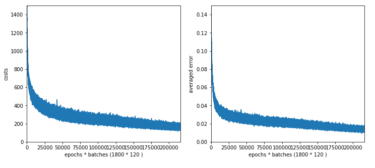
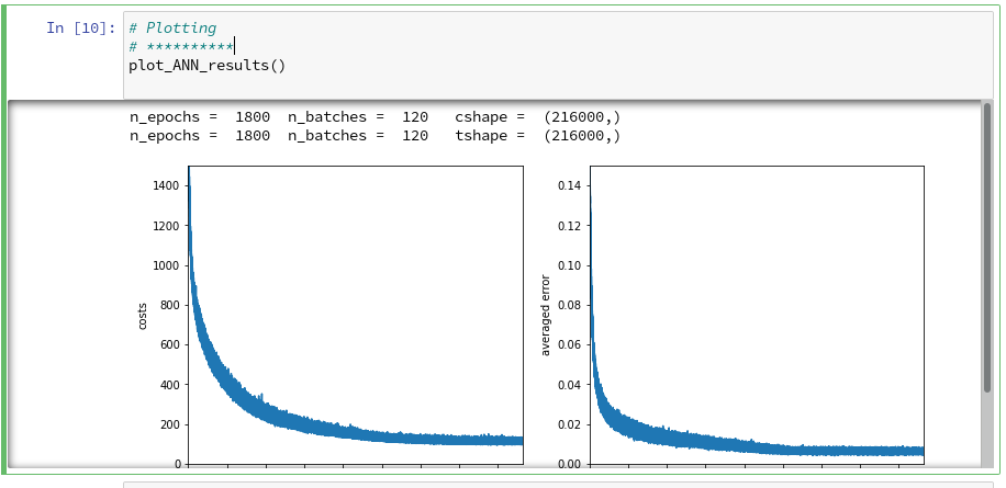
# Plotting
# **********
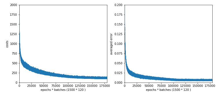
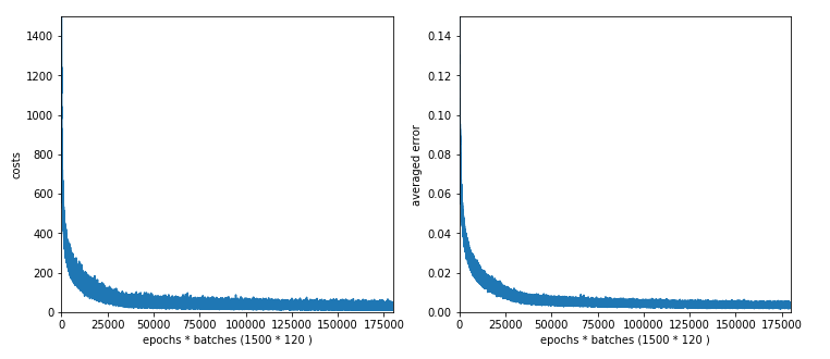
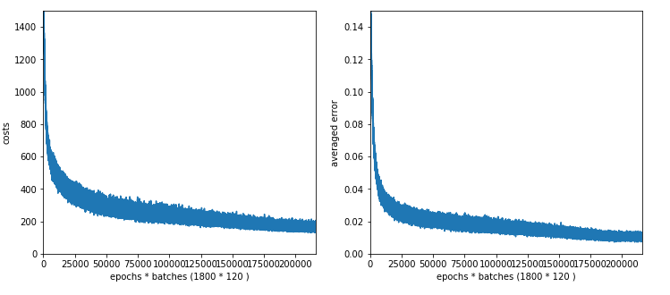
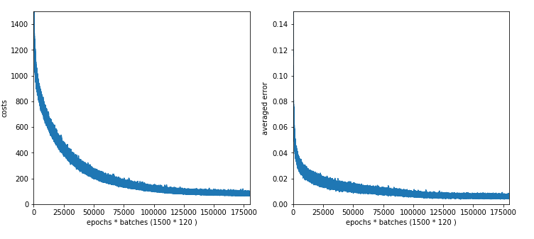
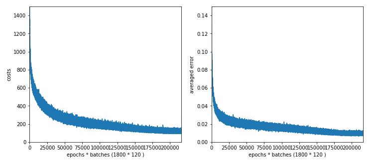
def plot_ANN_results():
num_epochs = ANN._n_epochs
num_batches = ANN._n_batches
num_tot = num_epochs * num_batches
cshape = ANN._ay_costs.shape
print("n_epochs = ", num_epochs, " n_batches = ", num_batches, " cshape = ", cshape )
tshape = ANN._ay_theta.shape
print("n_epochs = ", num_epochs, " n_batches = ", num_batches, " tshape = ", tshape )
#sizing
fig_size = plt.rcParams["figure.figsize"]
fig_size[0] = 12
fig_size[1] = 5
# Two figures
# -----------
fig1 = plt.figure(1)
fig2 = plt.figure(2)
# first figure with two plot-areas with axes
# --------------------------------------------
ax1_1 = fig1.add_subplot(121)
ax1_2 = fig1.add_subplot(122)
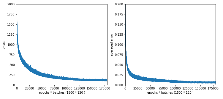
ax1_1.plot(range(len(ANN._ay_costs)), ANN._ay_costs)
ax1_1.set_xlim (0, num_tot+5)
ax1_1.set_ylim (0, 1500)
ax1_1.set_xlabel("epochs * batches (" + str(num_epochs) + " * " + str(num_batches) + " )")
ax1_1.set_ylabel("costs")
ax1_2.plot(range(len(ANN._ay_theta)), ANN._ay_theta)
ax1_2.set_xlim (0, num_tot+5)
ax1_2.set_ylim (0, 0.15)
ax1_2.set_xlabel("epochs * batches (" + str(num_epochs) + " * " + str(num_batches) + " )")
ax1_2.set_ylabel("averaged error")
The first function “predict_all_test_data()” allows us to create an array with the predicted values for all test data. This is based on a forward propagation of the full set of test data; so we handle some relatively big matrices here. The second function delivers prediction values for all training data; the operations of propagation algorithm involve even bigger matrices here. You will nevertheless experience that the calculations are performed very quickly. Prediction is much faster than training!
The third function “cm_analysis()” is not from me, but taken from Github Gist; see below. The fourth function “plot_ANN_results()” creates plots of the evolution of the cost function and the averaged error after training. We come back to these functions below.
To be able to use these functions we need to perform some more imports first. The full list of statements which we should place in the first Jupyter cell of our test notebook now reads:
import numpy as np
import numpy.random as npr
import math
import sys
import pandas as pd
from sklearn.datasets import fetch_openml
from sklearn.metrics import confusion_matrix
from scipy.special import expit
import seaborn as sns
from matplotlib import pyplot as plt
from matplotlib.colors import ListedColormap
import matplotlib.patches as mpat
import time
import imp
from mycode import myann
Note the new lines for the import of the “pandas” and “seaborn” libraries. Please inform yourself about the purpose of each library on the Internet.
Limited Accuracy
In the last article we performed some tests which showed a thorough robustness of our MLP regarding the MNIST datatset. There was some slight overfitting, but
playing around with hyper-parameters showed no extraordinary jump in “accuracy“, which we defined to be the percentage of correctly predicted records in the test dataset.
In general we can say that an accuracy level of 95% is what we could achieve within the range of parameters we played around with. Regression regularization (Lambda2 > 0) had some positive impact. A structural change to a MLP with just one layer did NOT give us a real breakthrough regarding CPU-time consumption, but when going down to 50 or 30 nodes in the intermediate layer we saw at least some reduction by up to 25%. But then our accuracy started to become worse.
Whilst we did our tests we measured the ANN’s “accuracy” by comparing the number of records for which our ANN did a correct prediction with the total number of records in the test data set. This is a global measure of accuracy; it averages over all 10 digits, i.e. all 10 classification categories. However, if we want to look a bit deeper into the prediction errors our MLP obviously produces it is, however, useful to introduce some more quantities and other measures of accuracy, which can be applied on the level of each output category.
Measures of accuracy, related quantities and classification errors for a specific category
The following quantities and basic concepts are often used in the context of ML algorithms for classification tasks. Predictions of our ANN will not be error free and thus we get an accuracy less than 100%. There are different reasons for this – and they couple different output categories. In the case of MNIST the output categories correspond to the digits 0 to 9. Let us take a specific output category, namely the digit “5”. Then there are two basic types of errors:
- The network may have predicted a “3” for a MNIST image record, which actually represents a “5” (according to the “y_train”-value for this record). This error case is called a “False Negative“.
- The network may have predicted a “5” for a MNIST image record, which actually represents a “3” according to its “y_train”-value. This error case is called a “False Positive“.
Both cases mark some difference between an actual and predicted number value for a MNIST test record. Technically, “actual” refers to the number value given by the related record in our array “ANN._y_test”. “Predicted” refers to the related record in an array “ay_prediction_test”, which our function “predict_all_test_data()” returns (see the code above).
Regarding our example digit “5” we obviously can distinguish between the following quantities:
- AN : The total number of all records in the test data set which actually correspond to our digit “5”.
- TP: The number of “True Positives”, i.e. the number of those cases correctly detected as “5”s.
- FP: The number of “False Positives”, i.e. the number of those cases where our ANN falsely predicts a “5”.
- FN: The number of “False Negatives”, i.e. the number of those cases where our ANN falsely predicts another digit than “5”, but where it actually should predict a “5”.
Then we can calculate the following ratios which all somehow measure “accuracy” for a specific output category:
-
Precision:TP / (TP + FP)
-
Recall:TP / ( TP + FN))
-
Accuracy:TP / AN
-
F1:TP / ( TP + 0.5*(FN + TP) )
A careful reader will (rightly) guess that the quantity “recall” corresponds to what we would naively define as “accuracy” – namely the ratio TP/AN.
From its definition it is clear that the quantity “F1” gives us a weighted average between the measures “precision” and “recall”.
How can we get these numbers for all 10 categories from our MLP after training ?
Confusion matrix
When we want to analyze our basic error types per category we need to look at the discrepancy between predicted and actual data. This suggests a presentation in form of a matrix with all for all possible category values both in x- and y-direction. The cells of such a matrix – e.g. a cell for an actual “5” and a predicted “3” – could e.g. be filled with the corresponding FN-number.
We will later on develop our own code to solve the task of creating and displaying such a matrix. But there is a nice guy called Runqi Yang who shared some code for precisely this purpose on GitHub Gist; see https://gist.github.com/hitvoice/36c…
We can use his suggested code as it is in our context. We have already presented it above in form of the function “cm_analysis()“, which uses the pandas and seaborn libraries.
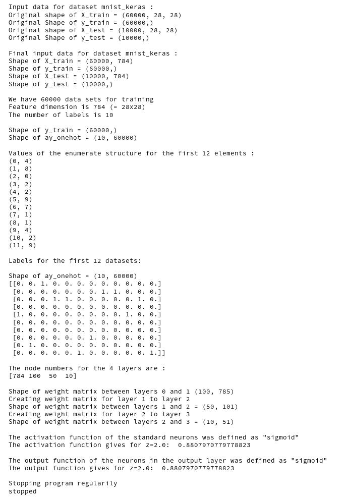
After a training run with the following parameters
try:
    ANN = myann.MyANN(my_data_set="mnist_keras", n_hidden_layers = 2,
                 ay_nodes_layers = [0, 70, 30, 0],
                 n_nodes_layer_out = 10,
                 my_loss_function = "LogLoss",
                 n_size_mini_batch = 500,
                 n_epochs = 1800,
                 n_max_batches = 2000,  # small values only for test runs
                 lambda2_reg = 0.2,
                 lambda1_reg = 0.0,
                 vect_mode = 'cols',
                 learn_rate = 0.0001,
                 decrease_const = 0.000001,
                 mom_rate   = 0.00005,
                 shuffle_batches = True,
                 print_period = 50,
                 figs_x1=12.0, figs_x2=8.0,
                 legend_loc='upper right',
                 b_print_test_data = True
                 )
except SystemExit:
    print("stopped")
we get
and
and eventually
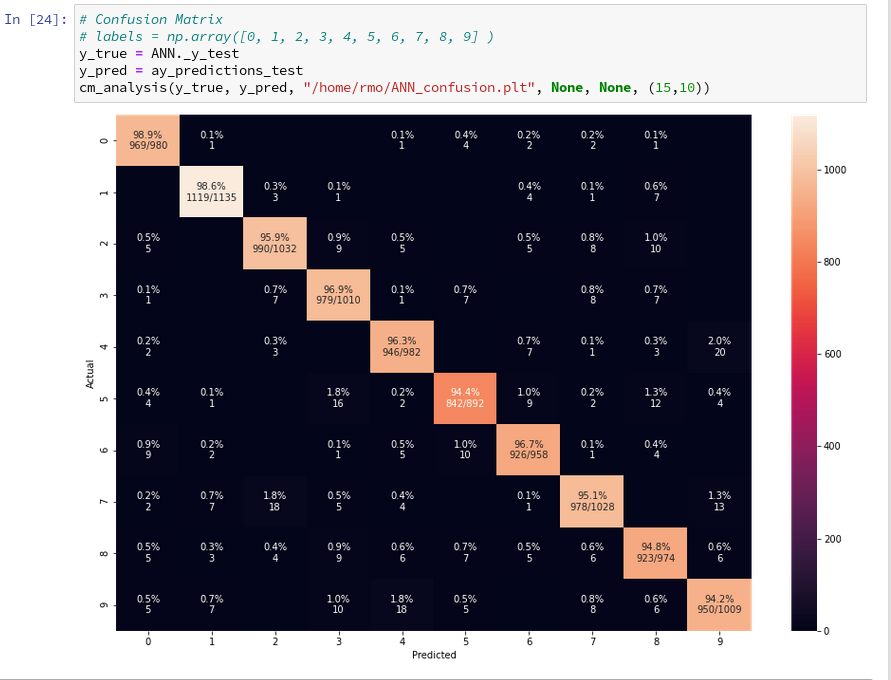
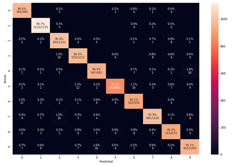
When I studied the last plot for a while I found it really instructive. Each of its cell outside the diagonal obviously contains the number of “False Negative” records for these two specific category values – but with respect to actual value.
What more do we learn from the matrix? Well, the numbers in the cells on the diagonal, in a row and in a
column are related to our quantities TP, FN and FP:
- Cells on the diagonal: For the diagonal we should find many correct “True Positive” values compared to the actual correct MNIST digits. (At least if all numbers are reasonably distributed across the MNIST dataset). We see that this indeed is the case. The ration of “True Positives” and the “Actual Positives” is given as a percentage and with the related numbers inside the respective cells on the diagonal.
- Cells of a row: The values in the cells of a row (without the cell on the diagonal) of the displayed matrix give us the numbers/ratios for “False Negatives” – with respect to the actual value. If you sum up the individual FN-numbers you get the total number of “False negatives”, which of course is the difference between the total number AN and the number TP for the actual category.
- Cells of a column: The column cells contain the numbers/ratios for “False Positives” – with respect to the predicted value. If you sum up the individual FN-numbers you get the total number of “False Positives” with respect to the predicted column value.
So, be a bit careful: A FN value with respect to an actual row value is a FP value with respect to the predicted column value – if the cell is one outside the diagonal!
All ratios are calculated with respect to the total actual numbers of data records for a specific category, i.e. a digit.
Looking closely we detect that our code obviously has some problems with distinguishing pictures of “5”s with pictures of “3”s, “6”s and “8”s. The same is true for “8”s and “3”s or “2s”. Also the distinction between “9”s, “3”s and “4”s seems to be difficult sometimes.
Does the confusion matrix change due to random initial weight values and mini-batch-shuffling?
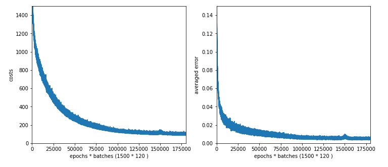
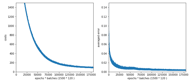
We have seen already that statistical variations have no big impact on the eventual accuracy when training converges to points in the parameter-space close to the point for the minimum of the overall cost-function. Statistical effects between to training runs stem in our case from statistically chosen initial values of the weights and the changes to our mini-batch composition between epochs. But as long as our training converges (and ends up in a global minimum) we should not see any big impact on the confusion matrix. And indeed a second run leads to:
The values are pretty close to those of the first run.
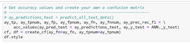
Precision, Recall values per digit category and our own confusion matrix
Ok, we now can look at the nice confusion matrix plot and sum up all the values in a row of the confusion matrix to get the total FN-number for the related actual digit value. Or sum up the entries in a column to get the total FP-number. But we want to calculate these values from the ANN’s prediction results without looking at a plot and summation handwork. In addition we want to get the data of the confusion matrix in our own Numpy matrix array independently of foreign code. The following box displays the code for two functions, which are well suited for this task:
# A class to print in color and bold
class color:
   PURPLE = '\033[95m'
   CYAN = '\033[96m'
   DARKCYAN = '\033[36m'
   BLUE = '\033[94m'
   GREEN = '\033[92m'
   YELLOW = '\033[93m'
   RED = '\033[91m'
   BOLD = '\033[1m'
   UNDERLINE = '\033[4m'
   END = '\033[
0m'

def acc_values(ay_pred_test, ay_y_test):
    ay_x = ay_pred_test
    ay_y = ay_y_test
    # -----
    #- dictionary for all false positives for all 10 digits
    fp = {}
    fpnum = {}
    irg = range(10)
    for i in irg:
        key = str(i)
        xfpi = np.where(ay_x==i)[0]
        fpi = np.zeros((10000, 3), np.int64)

        n = 0
        for j in xfpi:
            if ay_y[j] != i:
                row = np.array([j, ay_x[j], ay_y[j]])
                fpi[n] = row
                n+=1

        fpi_real   = fpi[0:n]
        fp[key]    = fpi_real
        fpnum[key] = fp[key].shape[0]

    #- dictionary for all false negatives for all 10 digits
    fn = {}
    fnnum = {}
    irg = range(10)
    for i in irg:
        key = str(i)
        yfni = np.where(ay_y==i)[0]
        fni = np.zeros((10000, 3), np.int64)

        n = 0
        for j in yfni:
            if ay_x[j] != i:
                row = np.array([j, ay_x[j], ay_y[j]])
                fni[n] = row
                n+=1

        fni_real = fni[0:n]
        fn[key] = fni_real
        fnnum[key] = fn[key].shape[0]

    #- dictionary for all true positives for all 10 digits
    tp = {}
    tpnum = {}
    actnum = {}
    irg = range(10)
    for i in irg:
        key = str(i)
        ytpi = np.where(ay_y==i)[0]
        actnum[key] = ytpi.shape[0]
        tpi = np.zeros((10000, 3), np.int64)

        n = 0
        for j in ytpi:
            if ay_x[j] == i:
                row = np.array([j, ay_x[j], ay_y[j]])
                tpi[n] = row
                n+=1

        tpi_real = tpi[0:n]
        tp[key] = tpi_real
        tpnum[key] = tp[key].shape[0]

    #- We create an array for the precision values of all 10 digits
    ay_prec_rec_f1 = np.zeros((10, 9), np.int64)
    print(color.BOLD + "Precision, Recall, F1, Accuracy, TP, FP, FN, AN" + color.END +"\n")
    print(color.BOLD + "i  ", "prec  ", "recall  ", "acc    ", "F1       ", "TP    ",
          "FP    ", "FN    ", "AN" + color.END)
    for i in irg:
        key = str(i)
        tpn = tpnum[key]
        fpn = fpnum[key]
        fnn = fnnum[key]
        an  = actnum[key]
        precision = tpn / (tpn + fpn)
        prec = format(precision, '7.3f')
        recall = tpn / (tpn + fnn)
        rec = format(recall, '7.3f')
        accuracy = tpn / an
        acc = format(accuracy, '7.3f')
        f1 = tpn / ( tpn + 0.5 * (fnn+fpn) )
        F1 = format(f1, '7.3f')
        TP = format(tpn, '6.0f')
        FP = format(fpn, '6.0f')
        FN = format(fnn, '6.0f')
        AN = format(an,  '6.0f')

        row = np.array([i, precision, recall, accuracy, f1, tpn, fpn, fnn, an])
        ay_prec_rec_f1[i] = row
        print (i, prec, rec, acc, F1, TP, FP, FN, AN)

    return tp, tpnum, fp, fpnum, fn, fnnum, ay_prec_rec_f1

def create_cf(ay_fn, ay_tpnum):
    ''' fn: array with false negatives row = np.array([j, x[j], y[j]])
    '''
    cf = np.zeros((10, 10), np.int64)
    rgi = range(10)
    rgj = range(10)
    for i in rgi:
        key = str(i)
        fn_i = ay_fn[key][ay_fn[key][:,2] == i]
        for j in rgj:
            if j!= i:
                fn_ij = fn_i[fn_i[:,1] == j]
                #print(i, j, fn_ij)
                num_fn_ij = fn_ij.shape[0]
                cf[i,j] = num_fn_ij
            if j==i:
                cf[i,j] = ay_tpnum[key]

    cols=["0", "1", "2", "3", "4", "5", "6", "7", "8", "9"]
    df = pd.DataFrame(cf, columns=cols, index=cols)
    # print( "\n", df, "\n")
    # df.style

    return cf, df
The first function takes a array with prediction values (later on provided externally
by our “ay_predictions_test”) and compares its values with those of an y_test array which contains the actual values (later provided externally by our “ANN._y_test”). Then it uses array-slicing to create new arrays with information on all error records, related indices and the confused category values. Eventually, the function determines the numbers for AN, TP, FP and FN (per digit category) and prints the gathered information. It also returns arrays with information on records which are “True Positives”, “False Positives”, “False Negatives” and the various numbers.
The second function uses array-slicing of the array which contains all information on the “False Negatives” to reproduce the confusion matrix. It involves Pandas to produce a styled output for the matrix.
Now you can run the above code and the following one in Jupyter cells – of course, only after you have completed a training and a prediction run:
For my last run I got the following data:
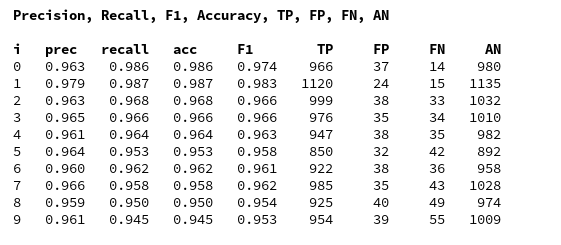
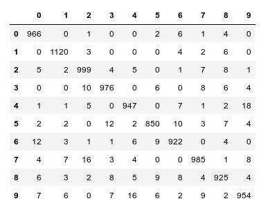
We again see that especially “5”s and “9”s have a problem with FNs. When you compare the values of the last printed matrix with those in the plot of the confusion matrix above, you will see that our code produces the right FN/FP/TP-values. We have succeeded in producing our own confusion matrix – and we have all values directly available in our own Numpy arrays.
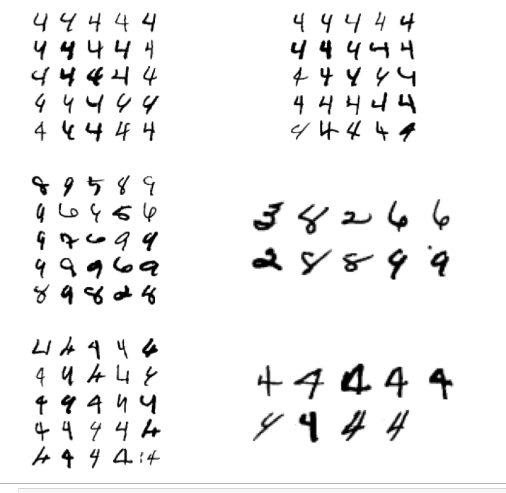
Some images of “4”-digits with errors
We can use the arrays which we created with functions above to get a look at the images. We use the function “plot_digits()” of Aurelien Geron at handson-ml2 chapter 03 on classification to plot several images in a series of rows and columns. The code is pretty easy to understand; at its center we find the matplotlib-function “imshow()”, which we have already used in other ML articles.
We again perform some array-slicing of the arrays our function “acc_values()” (see above) produces to identify the indices of images in the “X_test”-dataset we want to look at. We collect the first 50 examples of “true positive” images of the “4”-digit, then we take the “false positives” of the 4-digit and eventually the “fales negative” cases. We then plot the images in this order:
def plot_digits(instances, images_per_row=10, **options):
    size = 28
    images_per_row = min(len(instances), images_per_row)
    images = [instance.reshape(size,size) for instance in instances]
    n_rows = (len(instances) - 1) // images_per_row + 1
    row_images = []
    n_empty = n_rows * images_per_row - len(instances)
    images.append(np.zeros((size, size * n_empty)))
    for row in range(n_rows):
        rimages = images[row * images_per_row : (row + 1) * images_per_row]
        row_images.append(np.concatenate(rimages, axis=1))
    image = np.concatenate(row_images, axis=0)
    plt.imshow(image, cmap = mpl.cm.binary, **options)
    plt.axis("off")

ay_tp, ay_tpnum, ay_fp, ay_fpnum, ay_fn, ay_
fnnum, ay_prec_rec_f1 = \
    acc_values(ay_pred_test = ay_predictions_test, ay_y_test = ANN._y_test)

idx_act = str(4)

# fetching the true positives
num_tp = ay_tpnum[idx_act]
idx_tp = ay_tp[idx_act][:,[0]]
idx_tp = idx_tp[:,0]
X_test_tp = ANN._X_test[idx_tp]

# fetching the false positives
num_fp = ay_fpnum[idx_act]
idx_fp = ay_fp[idx_act][:,[0]]
idx_fp = idx_fp[:,0]
X_test_fp = ANN._X_test[idx_fp]

# fetching the false negatives
num_fn = ay_fnnum[idx_act]
idx_fn = ay_fn[idx_act][:,[0]]
idx_fn = idx_fn[:,0]
X_test_fn = ANN._X_test[idx_fn]

# plotting
# +++++++++++
plt.figure(figsize=(12,12))

# plotting the true positives
# --------------------------
plt.subplot(321)
plot_digits(X_test_tp[0:25], images_per_row=5 )
plt.subplot(322)
plot_digits(X_test_tp[25:50], images_per_row=5 )

# plotting the false positives
# --------------------------
plt.subplot(323)
plot_digits(X_test_fp[0:25], images_per_row=5 )
plt.subplot(324)
plot_digits(X_test_fp[25:], images_per_row=5 )

# plotting the false negatives
# ------------------------------
plt.subplot(325)
plot_digits(X_test_fn[0:25], images_per_row=5 )
plt.subplot(326)
plot_digits(X_test_fn[25:], images_per_row=5 )
The first row of the plot shows the (first) 50 “True Positives” for the “4”-digit images in the MNIST test data set. The second row shows the “False Positives”, the third row the “False Negatives”.
Very often you can guess why our MLP makes a mistake. However, in some cases we just have to acknowledge that the human brain is a much better pattern recognition machine than a stupid MLP 🙂 .
Conclusion
With the help of a “confusion matrix” it is easy to find out for which MNIST digit-images our algorithm has major problems. A confusion matrix gives us the necessary numbers of those digits (and their images) for which the MLP wrongly predicts “False Positives” or “False Negatives”.
We have also seen that there are three quantities – precision, recall, F1 – which are useful to describe the accuracy of a classification algorithm per classification category.
We have written some code to collect all necessary information about “confused” images into our own Numpy arrays after training. Slicing of Numpy arrays proved to be useful, and matplotlib helped us to visualize examples of the wrongly classified MNIST digit-images.
In the next article
A simple program for an ANN to cover the Mnist dataset – XII – accuracy evolution, learning rate, normalization
we shall extract some more information on the evolution of accuracy during training. We shall also make use of a “clustering” technique to reduce the number of input nodes.
Links
The python code of Runqi Yang (“hitvoice”) at gist.github.com for creating a plot of a confusion-matrix
Information on the function confusion_matrix() provided by sklearn.metrics
Information on the heatmap-functionality provided by “seaborn”
A python seaborn tutorial