A simple CNN for the MNIST dataset – VIII – filters and features – Python code to visualize patterns which activate a map strongly

Our series about a simple CNN trained on the MNIST data turns back to some coding.

A simple CNN for the MNIST dataset – VII – outline of steps to visualize image patterns which trigger filter maps
A simple CNN for the MNIST dataset – VI – classification by activation patterns and the role of the CNN’s MLP part
A simple CNN for the MNIST dataset – V – about the difference of activation patterns and features
A simple CNN for the MNIST dataset – IV – Visualizing the activation output of convolutional layers and maps
A simple CNN for the MNIST dataset – III – inclusion of a learning-rate scheduler, momentum and a L2-regularizer
A simple CNN for the MNIST datasets – II – building the CNN with Keras and a first test
A simple CNN for the MNIST datasets – I – CNN basics

In the last article I discussed an optimization algorithm which should be able to create images of pixel patterns which trigger selected feature maps of a CNN strongly. In this article we shall focus on the required code elements. I again want to emphasize that I apply and modify some basic ideas which I read in a book of F. Chollet and in a contribution of a guy called Mohamed to a discussion at kaggle.com (see my last article for references). A careful reader will notice differences not only with respect to coding; there are major differences regarding the normalization of intermediate data and the construction of input images. To motivate the latter point I first want to point out that OIPs are idealized technical abstractions and that not all maps may react to purely statistical data on short length scales.

Images of OIPs which trigger feature maps are artificial technical abstractions!

In the last articles I made an explicit distinction between two types of patterns which we can analyze in the context of CNNs:

  • FCP: A pattern which emerges within and across activation maps of a chosen (deep) convolutional layer due to filter operations which the CNN applied to a specific input image.
  • OIP: A pattern which is present within the pixel value distribution of an input image and to which a CNN map reacts strongly.

Regarding OIPs there are some points which we should keep in mind:

  • We do something artificial when we create an image of an elementary OIP pattern to which a chosen feature map reacts. Such an OIP is already an abstraction in the sense that it reflects an idealized pattern – i.e. a specific geometrical correlation between pixel values of an input image which passes a very specific filter combinations. We forget about all other figurative elements of the input image which may trigger other maps.
  • There is an additional subtle point regarding our present approach to OIP-visualization:
    Our algorithm – if it works – will lead to OIP images which trigger a
    map’s neurons maximally on average. What does “average” mean with respect to the image area? A map always covers the whole input image area. Now let us assume that a filter combination of lower layers reacts to an elementary pattern limited in size and located somewhere on the input image. But some filters or filter combinations may be capable of detecting such a pattern at multiple locations of an input image.
    One example would be a crossing of two relatively thin lines. Such a crossing could appear at many places in an input image. In fact, a trained CNN has seen several thousand images of handwritten “4”s where the crossing of the horizontal and the vertical line actually appeared at many different locations and may have learned about this when establishing filters. Under such conditions it is obvious that a map gets optimally activated if a relatively small elementary pattern appears multiple times within the image which our algorithm artificially constructs out of initial random data.
    So our algorithm will with a high probability lead to OIP images which consist of a combination or a superposition of elementary patterns at multiple locations. In this sense an OIP image constructed due to the rule of a maximum average activation is another type of idealization. In a real MNIST image the re-occurrence of elementary patterns may not be present at all. Therefore, we should be careful and not directly associate the visualization of a pattern created by our algorithm with an elementary OIP or “feature”.
  • The last argument can in some cases also be reverted: There may be unique large scale patterns which can only be detected by filters of higher (i.e. deeper) convolutional levels which filter coarsely and with respect to relatively large areas of the image. In our approach such unique patterns may only appear in OIP images constructed for maps of the deepest convolutional layer.

Independence of the statistical data of the input image?

In the last article I showed you already some interesting patterns for certain maps which emerged from randomly varying pixel values in an input image. The fluctuations were forced into patterns by the discussed optimization loop. An example of the resulting evolution of the pixel values is shown below: With more and more steps of the optimization loop an OIP-pattern emerges out of the initial “chaos”.

Images were taken at optimization steps 0, 9, 18, 36, 72, 144, 288, 599 of a loop. Convergence is given by a change of the loss values between two different steps divided by the present loss value :
3.6/41 => 3.9/76 => 3.3/143 => 2.3/240 => 0.8/346 => 0.15/398 => 0.03/418

As we work with gradient ascent in OIP detection a lower loss means a lower activation of the map.

If we change the wavelength of the initial input fluctuations we get a somewhat, though not fundamentally different result (actually with a lower loss value of 381):

This gives us confidence in the general usability of the method. However, I would like to point out that during your own experiments you may also experience the contrary:

For some maps and for some initial statistical input data varying at short length scales, only, the optimization process will not converge. It will not even start to do so. Instead you may experience a zero activation of the selected map during all steps of the optimization for a given random input.

You should not be too surprised by this fact. Our CNN was optimized to react to patterns present in written digits. As digits have specific elements (features?) as straight lines, bows, circles, line-crossings, etc., we should expect that not all input will trigger the activation of a selected map which reacts on pixel value variations at relatively large length scales. Therefore, it is helpful to be able to vary the statistical input pattern at different length scales when you start your hunt for a nice visualization of an OIP and/or elementary feature.

All in all we cannot exclude a dependency on the statistical initial input image fluctuations. Our algorithm will find a maximum with respect to the specific input data fluctuations presented to him. Due to this point we should always be aware of the fact that the visualizations produced by our algorithm will probably mark a local maximum in the multidimensional parameter or representation space – not a global one. But also a local maximum may reveal significant sub-structures a specific filter combination is sensitive to.

Libraries

To build a suitable code we need to import some libraries, which you first must install into your virtual Python environment:

  
import numpy as np
import scipy
import time 
import sys 
import math

from sklearn.preprocessing import StandardScaler
import tensorflow as tf
from tensorflow import keras as K
from tensorflow.python.keras import backend as B 
from tensorflow.keras import models
from tensorflow.keras import layers
from tensorflow.keras import regularizers
from tensorflow.keras import optimizers
from tensorflow.keras.optimizers import schedules
from tensorflow.keras.utils import to_categorical
from tensorflow.keras.datasets import mnist

from tensorflow.python.client import device_lib

import matplotlib as mpl
from matplotlib import pyplot as plt
from matplotlib.colors import ListedColormap
import matplotlib.patches as mpat 

import os 
from os import path as path


Basic code elements to construct OIP patterns from statistical input image data

To develop some code for OIP visualizations we follow the outline of steps discussed in the last article. To encapsulate the required functionality we set up a Python class. The following code fragment gives an overview about some variables which we are going to use. In the comments and explanations I sometimes used the word “reference” to mark a difference between

  • addresses to some intermediate Tensorflow 2 [TF2] objects handled by a “watch()“-method of TF2’s GradientTape-object for eager calculation of gradients
  • and eventual return objects (of a function based on keras’ backend) filled with values which we can directly use during the optimization iterations for corrections.

This is only a reminder of complex internal TF2 background operations based on complex layer models; I do not want to stress any difference in the sense of pointers and objects. Actually, I do not even know the precise programming patterns used behind TF2’s watch()-mechanism; but according to the documentation it basically records all operations involving the “watched” objects. The objective is the ability to produce gradient values of defined functions with respect to any variable changes instantaneously in eager execution later on.

 
# class to produce images of OIPs for a chosen CNN-map
# ****************************
***************************
class My_OIP:
    '''
    Version 0.2, 01.09.2020
    ~~~~~~~~~~~~~~~~~~~~~~~~~
    This class allows for the creation and the display of OIP-patterns 
    to which a selected map of a CNN-model reacts   
    
    Functions:
    ~~~~~~~~~~
    1) _load_cnn_model()             => load cnn-model
    2) _build_oip_model()            => build an oip-model to create OIP-images
    3) _setup_gradient_tape()        => Implements TF2 GradientTape to watch input data
                                        for eager gradient calculation
    4) _oip_strat_0_optimization_loop():
                                     => Method implementing a simple strategy to create OIP-images 
                                        based on superposition of random data on large distance scales
    5) _oip_strat_1_optimization_loop():
       (NOT YET DEVELOPED)           => Method implementing a complex strategy to create OIP-images 
                                        based on partially evolved intermediate image 
                                        getting enriched by small scale fluctuations
    6) _derive_OIP():                => Method used externally to start the creation of 
                                        an OIP for a chosen map 
    7) _build_initial_img_data()     => Method to construct an initial image based on 
                                        a superposition by random date on 4 different length scales 
    
    
    Requirements / Preconditions:
    ~~~~~~~~~~~~~~~~~~~~~~~~~~~~~
    In the present version 
    * a CNN-model is assumed which works with standardized (!) input images,
    * a CNN-Modell trained on MNIST data is assumed ,
    * exactly 4 length scales for random data fluctations are used
      to compose initial statistical image data 
      (roughly with a factor of 2 between them) 
      
    
    '''
    def __init__(self, cnn_model_file = 'cnn_best.h5', 
                 layer_name = 'Conv2D_3', map_index = 0, 
                 img_dim = 28, 
                 b_build_oip_model = True  
                ): 
        '''
        Input: 
        ~~~~~~
            cnn_model_file:     Name of a file containing  a full CNN-model
                                can later be overwritten by _load_cnn_model()
            layer_name:         We can define a layer name we are interested in already when starting; s. below
            map_index:          We may define a map we are interested in already when starting; s. below
            img_dim:            The dimension of the assumed quadratic images 
        
        Major internal variables:
        **************************
            _cnn_model:             A reference to the CNN model object
            _layer_name:            The name of convolutional layer 
                                    (can be overwritten by method _build_oip_model() ) 
            _map_index:             index of the map in the layer's output array 
                                    (can later be overwritten by other methods) 
            _r_cnn_inputs:          A reference to the input tensor of the CNN model (here: 1 image - NOT a batch of images)
            _layer_output:          Tensor with all maps of a certain layer
           
            _oip_submodel:          A new model connecting the input of the cnn-model with a certain map
            
            _tape:                  An instance of TF2's GradientTape-object 
                                    Watches input, output, loss of a model 
                                    and calculates gradients in TF2 eager mode 
            _r_oip_outputs:         A reference to the output of the new OIP-model 
            _r_oip_grads:           Reference to gradient tensors for the new OIP-model 
            _r_oip_loss:            Reference to a loss 
defined by operations on the OIP-output  
            _val_oip_loss:          Reference to a loss defined by operations on the OIP-output  
            
            _iterate:               Keras backend function to invoke the new OIP-model 
                                    and calculate both loss and gradient values (in TF2 eager mode) 
                                    This is the function to be used in the optimization loop for OIPs
            
            Parameters controlling the optimization loop:
            ~~~~~~~~~~~~~~~~~~~~~~~~~~~~~~~~~~~~~~~~~~~
            _oip_strategy:          0, 1 - There are two strategies to evolve OIP patterns out of statistical data - only the first strategy is supported in this version  
                                    0: Simple superposition of fluctuations at different length scales
                                    1: Evolution over partially evolved images based on longer scale variations 
                                       enriched with fluctuations on shorter length scales 
                                    Both strategies can be combined with a precursor calculation 
            
            
            _b_oip_precursor:       True/False - Use a precursor analysis of long range variations 
                                    regarding loss => search for optimum variations for a given map
                                    (Some initial input images do not trigger a map at all or 
                                    sub-optimally => We test out multiple initial fluctuation patterns). 
            
            _ay_epochs:             A list of 4 optimization epochs to be used whilst 
                                    evolving the img data via strategy 1 and intermediate images 
            _n_epochs:              Number of optimization epochs to be used with strategy 0 
            
            _n_steps:               Defines at how many intermediate points we show images and report 
                                    on the optimization process 
            
            _epsilon:               Factor to control the amount of correction imposed by 
                                    the gradient values of the OIP-model 
            
            Input image data of the OIP-model and references to it 
            ~~~~~~~~~~~~~~~~~~~~~~~~~~~~~~~~~~
            _initial_precursor_img  The initial image to start a precursor optimization with.
                                    Would normally be an image of only long range fluctuations. 
            _precursor_image:       The evolved image updated during the precursor loop 
            
            _initial_inp_img_data:  A tensor representing the data of the input image 
            _inp_img_data:          A tensor representing the data of the input img during optimization  
            _img_dim:               We assume quadratic images to work with 
                                    with dimension _img_dim along each axis
                                    For the time being we only support MNIST images 
            
            Parameters controlling the composition of random initial image data 
            ~~~~~~~~~~~~~~~~~~~~~~~~~~~~~~~~~~~~~~~~~~~
            _li_dim_steps:          A list of the intermediate dimensions for random data;
                                    these data are smoothly scaled to the image dimensions 
            _ay_facts:              A Numpy array of 4 factors to control the amount of 
                                    contribution of the statistical variations 
                                    on the 4 length scales to the initial image
                                   
        '''    
        
        # Input data and variable initializations
        # ****************************************
        
        # the model 
        self._cnn_model_file = cnn_model_file
        self._
cnn_model      = None 
        
        # the layer 
        self._layer_name = layer_name
        # the map 
        self._map_index  = map_index
        
        # References to objects and the OIP sub-model
        # ~~~~~~~~~~~~~~~~~~~~~~~~~~~~~~
        self._r_cnn_inputs  = None # reference to input of the CNN_model
                                   # also used in the OIP-model  
        
        self._layer_output  = None
        self._oip_submodel  = None
        
        self._tape          = None # TF2 GradientTape variable
        # some "references"
        self._r_oip_outputs = None # output of the OIP-submodel to be watched 
        self._r_oip_grads   = None # gradients determined by GradientTape   
        self._r_oip_loss    = None 
        # respective values
        self._val_oip_grads = None
        self._val_oip_loss  = None
        
        # The Keras function to produce concrete outputs of the new OIP-model  
        self._iterate       = None
        
        # The strategy to produce an OIP pattern out of statistical input images 
        # ~~~~~~~~~~~~~~~~~~~~~~~~~--------~~~~~~
        # 0: Simple superposition of fluctuations at different length scales 
        # 1: Move over 4 interediate images - partially optimized 
        self._oip_strategy = 0
        
        # Parameters controlling the OIP-optimization process 
        # ~~~~~~~~~~~~~~~~~~~~~~~~~--------~~~~~~
        # Use a precursor analysis ? 
        self._b_oip_precursor = False
       
        # number of epochs for optimization strategy 1
        self._ay_epochs    = np.array((20, 40, 80, 400))
        len_epochs         = len(self._ay_epochs)

        # number of epochs for optimization strategy 0
        self._n_epochs     = self._ay_epochs[len_epochs-1]   
        self._n_steps      = 7   # divides the number of n_epochs into n_steps 
                                 # to produce intermediate outputs
        
        # size of corrections by gradients
        self._epsilon       = 0.01 # step-size for gradient correction
        
        
        # Input images and references to it 
        # ~~~~~~~~
        # precursor image
        self._initial_precursor_img = None
        self._precursor_img         = None
        # The evetually used input image - a superposition of initial random fluctuations
        self._initial_inp_img_data  = None  # The initial data constructed 
        self._inp_img_data          = None  # The data used and varied for optimization 
        # image dimension
        self._img_dim               = img_dim   # = 28 => MNIST images for the time being 
        
        
        # Parameters controlling the setup of an initial image 
        # ~~~~~~~~~~~~~~~~~~~~~~~~~--------~~~~~~~~~~~~~~~~~~~
        # The length scales for initial input fluctuations
        self._li_dim_steps = ( (3, 3), (7,7), (14,14), (28,28) )
        # Parameters for fluctuations  - used both in strategy 0 and strategy 1  
        self._ay_facts     = np.array( (0.5, 0.5, 0.5, 0.5) )
        
        
        # ********************************************************
        # Model setup - load the cnn-model and build the oip-model
        # ************
        
        if path.isfile(self._cnn_model_file): 
            # We trigger the initial load of a model 
            self._load_cnn_model(file_of_cnn_model = self._cnn_model_file, b_print_cnn_model = True)
            # We trigger the build of a new sub-model based on the CNN model used for OIP search 
            self._build_oip_model(layer_name = self._layer_name, b_print_oip_model = True ) 
        else:
            print("<\nWarning: The standard file " + self._cnn_model_file + 
                  " for the cnn-model could not be found!\n " + 
                  " Please use method _load_cnn_model() to load 
a valid model")
            
        return


The purpose of most of the variables will become clearer as we walk though the class’s methods below.

Loading the original trained CNN model

Let us say we have a trained CNN-model with all final weight parameters for node-connections saved in some h5-file (see the 4th article of this series for more info). We then can load the CNN-model and derive sub-models from its layer elements. The following method performs the loading task for us:

 
    #
    # Method to load a specific CNN model
    # **********************************
    def _load_cnn_model(self, file_of_cnn_model='cnn_best.h5', b_print_cnn_model=True ):
        
        # Check existence of the file
        if not path.isfile(self._cnn_model_file): 
            print("<\nWarning: The file " + file_of_cnn_model + 
                  " for the cnn-model could not be found!\n" + 
                  "Please change the parameter \"file_of_cnn_model\"" + 
                  " to load a valid model")

        # load the CNN model 
        self._cnn_model_file = file_of_cnn_model
        self._cnn_model = models.load_model(self._cnn_model_file)

        # Inform about the model and its file file 7
        # ~~~~~~~~~~~~~~~~~~~~~~~~~~~
        print("Used file to load a ´ model = ", self._cnn_model_file)
        # we print out the models structure
        if b_print_cnn_model:
            print("Structure of the loaded CNN-model:\n")
            self._cnn_model.summary()

        # handle/references to the models input => more precise the input image 
        # ~~~~~~~~~~~~~~~~~~~~~~~~~~~~~~~~~~~~
        #    Note: As we only have one image instead of a batch 
        #    we pick only the first tensor element!
        #    The inputs will be needed for buildng the oip-model 
        self._r_cnn_inputs = self._cnn_model.inputs[0]  # !!! We have a btach with just ONE image 
        
        # print out the shape - it should be known fro the original cnn-model
        print("shape of cnn-model inputs = ", self._r_cnn_inputs.shape)
        
        return

 
Actually, I used this function already in the class’ “__init__()”-method – provided the standard file for the last CNN exists. (In a more advanced version you would in addition check that the name of the standard CNN-model meets your expectations.)

The code is straightforward. You see that the structure of the original CNN-model is printed out if requested by the user.

Note also that we assigned the first element of the input tensor of the CNN-model, i.e. a single image tensor, to the variable “self._r_cnn_inputs”. This tensor will become a major ingredient in a new Keras model which we are going to build in a minute and which we shall use to calculate gradient components of a loss function with respect to all pixel values of the input image. The gradient’s component values will in turn be used during gradient ascent to correct the pixel values. Repeated corrections should lead to a systematic approach of a maximum of our loss function, which describes the map’s activation. (Remember: Such a maximum may depend on the input image fluctuations).

Build a new Keras model based on the input tensor and a chosen layer

The next method is more interesting. We need to build a new Keras layer “model” based on the input layer and a deeper layer of the original CNN-model. (We already used the same kind of “trick” when we tried to visualize the activation output of a convolutional layer of the CNN.)

 
    #
    # Method to construct a model to optimize input for OIP-detection 
    # 
***************************************
    def _build_oip_model(self, layer_name = 'Conv2D_3', b_print_oip_model=True ): 
        '''
        We need a Conv layer to build a working model for input image optimization. 
        We get the Conv layer by the layer's name. 
        The new model connects the first input element of the CNN to 
        the output maps of the named Conv layer CNN 
        '''
        # free some RAM - hopefully 
        del self._oip_submodel
        
        self._layer_name = layer_name
        if self._cnn_model == None: 
            print("Error: cnn_model not yet defined.")
            sys.exit()
        # We build a new model based ion the model inputs and the output 
        self._layer_output = self._cnn_model.get_layer(self._layer_name).output
        
        # We do not acre at the moment about the composition of the input 
        # We trust in that we handle only one image - and not a batch
        model_name = "mod_oip__" + layer_name 
        self._oip_submodel = models.Model( [self._r_cnn_inputs], [self._layer_output], name = model_name)                                    
        
        # We print out the oip model structure
        if b_print_oip_model:
            print("Structure of the constructed OIP-sub-model:\n")
            self._oip_submodel.summary()
        return

 
We use the tensor for a single input image and the output of layer (= a collection of maps) of the original CNN-model as the definition elements of the new Keras model.

TF2’s GradientTape() – watch the change of variables which have an impact on model gradients and the loss function

What do we have so far? We have defined a new Keras model connecting input and output data of a layer of the original model. TF2 can determine related gradients by the node connections defined in the original model. However, we cannot rely on a graph analysis by Tensorflow as we were used to with TF1. TF2 uses eager mode – i.e. it calculates gradients directly. What does “directly” mean? Well – as soon as changes to variables occur which have an impact on the gradient values. This in turn means that “something” has to watch out for such changes. TF2 offers a special object for this purpose: tf.GradientTape. See:
https://www.tensorflow.org/guide/eager
https://www.tensorflow.org / api_docs/python/tf/GradientTape

So, as a next step, we set up a method to take care of “GradientTape()”.

    #
    # Method to watch gradients 
    # *************************
    def _setup_gradient_tape(self):
        '''
        For TF2 eager execution we need to watch input changes and trigger gradient evaluation
        '''   
        # Working with TF2 GradientTape
        self._tape = None
        
        # Watch out for input, output variables with respect to gradient chnages
        with tf.GradientTape() as self._tape: 
            # Input
            # ~~~~~~~
            self._tape.watch(self._r_cnn_inputs)
            # Output 
            # ~~~~~~~
            self._r_oip_outputs = self._oip_submodel(self._r_cnn_inputs)
            
            # Loss 
            # ~~~~~~~
            self._r_oip_loss = tf.reduce_mean(self._r_oip_outputs[0, :, :, self._map_index])
            print(self._r_oip_loss)
            print("shape of oip_loss = ", self._r_oip_loss.shape)

 
Note that the loss definition included in the code fragment is specific for a chosen map. This implies that we have to call this method every time we chose a different map for which we want to create OIP visualizations.

The advantage of the above code element is that “_tape()” can produce gradient values for the relation of the input data and loss data of a model automatically whenever we change the input image data. Gradient values can be called by

  self._r_oip_grads  = self._tape.gradient(self._r_oip_loss, self._r_cnn_inputs)

Gradient ascent

As already discussed in my last article we apply a gradient ascent method to our “loss” function whose outcome rises with the activation of the neurons of a map. The following code sets up a method which first calls “_setup_gradient_tape()” and afterwards applies a normalization to the gradient values which “_tape()” produces. It then defines a convenience function and eventually calls a method which runs the optimization loop.

    #        
    # Method to derive OIP from a given initial input image
    # ********************
    def _derive_OIP(self, map_index = 1, n_epochs = None, n_steps = 4, 
                          epsilon = 0.01, 
                          conv_criterion = 5.e-4, 
                          b_stop_with_convergence = False ):
        '''
        V0.3, 31.08.2020
        This method starts the process of producing an OIP of statistical input image data
        
        Requirements:    An initial input image with statistical fluctuations of pixel values 
        -------------    must have been created. 
        
        Restrictions:    This version only supports the most simple strategy - "strategy 0":  
        -------------    Optimize in one loop - starting from a superposition of fluctuations
                         No precursor, no intermediate evolution of input image data 
        
        Input:
        ------
        map_index:       We can chose a map here       (overwrites previous settings)
        n_epochs:        Number of optimization steps  (overwrites previous settings) 
        n_steps:         Defines number of intervals (with length n_epochs/ n_steps) for reporting
                         This number also sets a requirement for providing n_step external axis-frames 
                         to display intermediate images of the emerging OIP  
                         => see _oip_strat_0_optimization_loop()
        epsilon:         Size for corrections by gradient values
        conv_criterion:  A small threshold number for (difference of loss-values / present loss value )
        b_stop_with_convergence: 
                         Boolean which decides whether we stop a loop if the conv-criterion is fulfilled
                         
        '''
        self._map_index = map_index
        self._n_epochs  = n_epochs   
        self._n_steps   = n_steps
        self._epsilon   = epsilon
        
        # number of epochs for optimization strategy 0 
        # ~~~~~~~~~~~~~~~~~~~~~~~~~~~~~~~~~~~~~~~~~~~~~~
        if n_epochs == None:
            len_epochs = len(self._ay_epochs)
            self._n_epochs   = self._ay_epochs[len_epochs-1]
        else: 
            self._n_epochs = n_epochs
            
        # Rest some variables  
        self._val_oip_grads = None
        self._val_oip_loss  = None 
        self._iterate       = None 
        
        # Setup the TF2 GradientTape watch
        # ~~~~~~~~~~~~~~~~~~~~~~~~~~~~~~~~~~~~~~~~~~~~~~~~~~~
        self._setup_gradient_tape()
        print("GradientTape watch activated ")
    
        # Gradient handling - so far we only deal with addresses 
        # ~~~~~~~~~~~~~~~~~~
        self._r_oip_grads  = self._tape.gradient(self._r_oip_loss, self._r_cnn_inputs)
        #print("shape of grads = ", self._r_oip_grads.shape)
        
        # normalization of the gradient 
        self._r_oip_grads /= (B.sqrt(B.mean(B.
square(self._r_oip_grads))) + 1.e-7)
        #grads = tf.image.per_image_standardization(grads)
        
        # define an abstract recallable Keras function 
        # producing loss and gradients for corrected img data 
        # the first list of addresses points to the input data, the last to the output data 
        self._iterate = B.function( [self._r_cnn_inputs], [self._r_oip_loss, self._r_oip_grads] )
        
        # get the initial image into a variable for optimization 
        self._inp_img_data = None
        self._inp_img_data = self._initial_inp_img_data
        
        # Optimization loop for strategy 0 
        # ~~~~~~~~~~~~~~~~~~~~~~~~~~~~~~~~
        if self._oip_strategy == 0: 
            self._oip_strat_0_optimization_loop( conv_criterion = conv_criterion, 
                                                b_stop_with_convergence = b_stop_with_convergence )


Gradient value normalization is done here with respect to the L2-norm of the gradient. I.e., we adjust the length of the gradient to a unit length. Why does such a normalization help us with respect to convergence? You remember from a previous article series about MLPs that we had to care about a reasonable balance of an adaptive application of gradient values and a systematic reduction of the learning rate when approaching the global minimum of a cost function. The various available adaptive gradient methods care about speed and a proper deceleration of the steps by which we move across the cost hyperplane. When we approached a minimum we needed to care about overshooting. In our present gradient ascent case we have no such adaptive fine-tuning available. What we can do, however, is to control the length of the gradient vector such that changes remain of the same order as long as we do not change the step-size factor (epsilon). I.e.:

  • We do not wildly accelerate our path on the loss hyperplane when some local pixel areas want to drive us into a certain direction.
  • We reduce the chance of creating pixel values out of normal boundaries.

The last point fits well with a situation where the CNN has been trained on normalized or standardizes input images. Due to the normalization the size of pixel value corrections now depends significantly on the factor “epsilon”. We should choose it small enough with respect to the pixel values.

Another interesting statement in the above code fragment is

        self._iterate = B.function( [self._r_cnn_inputs], [self._r_oip_loss, self._r_oip_grads] )

Here we use the Keras Backend to define a convenience function which relates input data with dependent outputs, whose calculations we previously defined by suitable statements. The list which is used as the first parameter of this function “_iterate()” defines the input variables, the list used as a second parameter defines the output variables which will internally be calculated via the GradientTape-functionality defined before. The “_iterate()”-function makes it much easier for us to build the optimization loop.

The optimization loop for the construction of images that visualize OIPs and features

The optimization loop must systematically correct the pixel values to approach a maximum of the loss function. The following method “_oip_strat_0_optimization_loop()” does this job for us. (The “0” in the method’s name refers to a first simple approach.)

    #        
    # Method to optimize an emerging OIP out of statistical input image data 
    # (simple strategy - just optimize, no precursor, no intermediate pattern evolution 
    # ********************************
    def _oip_strat_0_optimization_loop(self, conv_criterion = 5.e-4, 
                                            b_stop_with_
convergence = False ):
        
        '''
        V 0.2, 28.08.2020 
        
        Purpose: 
        This method controls the optimization loop for OIP reconstruction of an initial 
        input image with a statistical distribution of pixel values. 
        It also provides intermediate output in the form of printed data and images.
        
        Parameter: 
        conv_criterion:  A small threshold number for (difference of loss-values / present loss value )
        b_stop_with_convergence: 
                         Booelan which decides whether we stop a loop if the conv-criterion is fulfilled
        
        
        This method produces some intermediate output during the optimization loop in form of images.
        It uses an external grid of plot frames and their axes-objects. The addresses of the 
        axis-objects must provided by an external list "li_axa[]".  
        We need a seqence of >= n_steps axis-frames length(li_axa) >= n_steps).    
        With Jupyter the grid for plots can externally be provided by statements like 
        
        # figure
        # -----------
        #sizing
        fig_size = plt.rcParams["figure.figsize"]
        fig_size[0] = 16
        fig_size[1] = 8
        fig_a = plt.figure()
        axa_1 = fig_a.add_subplot(241)
        axa_2 = fig_a.add_subplot(242)
        axa_3 = fig_a.add_subplot(243)
        axa_4 = fig_a.add_subplot(244)
        axa_5 = fig_a.add_subplot(245)
        axa_6 = fig_a.add_subplot(246)
        axa_7 = fig_a.add_subplot(247)
        axa_8 = fig_a.add_subplot(248)
        li_axa = [axa_1, axa_2, axa_3, axa_4, axa_5, axa_6, axa_7, axa_8]
        
        '''
        
        # Check that we really have an input image tensor
        if ( (self._inp_img_data == None) or 
             (self._inp_img_data.shape[1] != self._img_dim) or 
             (self._inp_img_data.shape[2] != self._img_dim) ) :
            print("There is no initial input image or it does not fit dimension requirements (28,28)")
            sys.exit()
        
        # Print some information
        print("*************\nStart of optimization loop\n*************")
        print("Strategy: Simple initial mixture of long and short range variations")
        print("Number of epochs = ", self._n_epochs)
        print("Epsilon =  ", self._epsilon)
        print("*************")
        
        # some initial value
        loss_old = 0.0
       
        # Preparation of intermediate reporting / img printing
        # --------------------------------------
        # Number of intermediate reporting points during the loop 
        steps = math.ceil(self._n_epochs / self._n_steps )
        # Logarithmic spacing of steps (most things happen initially)
        n_el = math.floor(self._n_epochs / 2**(self._n_steps) ) 
        li_int = []
        for j in range(self._n_steps):
            li_int.append(n_el*2**j)
        print("li_int = ", li_int)
        # A counter for intermediate reporting  
        n_rep = 0
        # Array for intermediate image data 
        li_imgs = np.zeros((self._img_dim, self._img_dim, 1), dtype=np.float32)
        
        # Convergence? - A list for steps meeting the convergence criterion
        # ~~~~~~~~~~~~
        li_conv = []
        
        
        # optimization loop 
        # *******************
        # A counter for steps with zero loss and gradient values 
        n_zeros = 0
        
        for j in range(self._n_epochs):
            
            # Get output values of our Keras iteration function 
            # ~~~~~~~~~~~~~~~~~~~
            self._val_oip_loss, self._val_oip_grads = self._iterate([self._inp_img_data])
            
            # loss difference to last step - shuold steadily become smaller 
            loss_diff = self._
val_oip_loss - loss_old 
            #print("loss_val = ", loss_val)
            #print("loss_diff = ", loss_diff)
            loss_old = self._val_oip_loss
            
            if j > 10 and (loss_diff/(self._val_oip_loss + 1.-7)) < conv_criterion:
                li_conv.append(j)
                lenc = len(li_conv)
                # print("conv - step = ", j)
                # stop only after the criterion has been met in 4 successive steps
                if b_stop_with_convergence and lenc > 5 and li_conv[-4] == j-4:
                    return
            
            grads_val     = self._val_oip_grads
            # the gradients average value 
            avg_grads_val = (tf.reduce_mean(grads_val)).numpy()
            
            # Check if our map reacts at all
            # ~~~~~~~~~~~~~~~~~~~~~~~~~~~~~~~~
            if self._val_oip_loss == 0.0 and avg_grads_val == 0.0:
                print( "0-values, j= ", j, 
                       " loss = ", self._val_oip_loss, " avg_loss = ", avg_grads_val )
                n_zeros += 1
            
            if n_zeros > 10: 
                print("More than 10 times zero values - Try a different initial random distribution of pixel values")
                return
            
            # gradient ascent => Correction of the input image data 
            # ~~~~~~~~~~~~~~~
            self._inp_img_data += grads_val * self._epsilon
            
            # Standardize the corrected image - we won't get a convergence otherwise 
            # ~~~~~~~~~~~~~~~~~~~~~~~~~~~~~~~
            self._inp_img_data = tf.image.per_image_standardization(self._inp_img_data)
            
            # Some output at intermediate points 
            #     Note: We us logarithmic intervals because most changes 
            #           appear in the intial third of the loop's range  
            if (j == 0) or (j in li_int) or (j == self._n_epochs-1) :
                # print some info 
                print("\nstep " + str(j) + " finalized")
                #print("Shape of grads = ", grads_val.shape)
                print("present loss_val = ", self._val_oip_loss)
                print("loss_diff = ", loss_diff)
                # display the intermediate image data in an external grid 
                imgn = self._inp_img_data[0,:,:,0].numpy()
                #print("Shape of intermediate img = ", imgn.shape)
                li_axa[n_rep].imshow(imgn, cmap=plt.cm.viridis)
                # counter
                n_rep += 1
         
        return

 
The code is easy to understand: We use our convenience function “self._iterate()” to produce actual loss and gradient values within the loop. Then we change the pixel values of our input image and feed the changed image back into the loop. Note the positive sign of the correction! All complicated gradient calculations are automatically and “eagerly” done internally thanks to “GradientTape”.

We said above that we limited the gradient values. How big is the size of the resulting corrections compared to the image data? If and when we use standardized image data and scale our gradient to unit length size then the relative size of the changes are of the order of the step size “epsilon” for the correction. In our case we set epsilon to 5.e-4.

The careful reader has noticed that I standardized the image data after the correction with the (normalized) gradient. Well, this step proved to be absolutely necessary to get convergence in the sense that we really approach an extremum of the cost function. Reasons are:

  • My CNN was trained on standardized MNIST input images.
  • We did not include any normalization layers into our CNN.
  • Without counter-measures our normalized gradient values would eventually drive unlimited activation
    values.

The last point deserves some explanation:

We used the ReLU-function as the activation function of nodes in the inner layers of our CNN. For positive input values ReLU actually is a linear function. Now let us assume that we have found a rather optimal input pattern which via a succession of basically linear operations drives an activation pattern of a map’s neurons. What happens if we just add constant small values to each pixel per iteration step? The output values after the sequence of linear transformations will just grow! With our method and the ReLU activation function we walk around a surface until we reach a linear ramp and climb it up. Without compensatory steps we will not find a real maximum because there is none. The situation is very different at the convolutional layers than at the eventual output layer of the CNN’s MLP-part.

You may ask yourself why we experienced nothing of this during the classification training? First answer: We did not optimize input data but weights during the training. Second answer: During training we did NOT maximize potentially unbound activation values but minimized a cost function based on output values of the last a MLP-layer. And these values were produced by a sigmoid function! The sigmoid function limits any input to the range ]0, +1[. In addition, the cost function (categorial_crossentropy) is designed to be convex for deviations of limited calculated values from a limited target vector.

The consequence is that we have to limit the values of the (corrected) input data and the related gradients in our present optimization procedure at the same time! This is done by the standardization of the image data. Remember that the correction values are around of the relative order of 5.e-4. In the end this is the order of the fluctuations which are unavoidable in the final OIP image; but now we have a chance to converge to a related small region around a real maximum.

The last block in the code deals with intermediate output – not only printed data on the loss function but also in form of intermediate images of the hopefully emerging pattern. These images can be provided in an external grid of figures in e.g. a Jupyter environment. The important point is that we define a suitable number of Matplotlib’s axis-objects and deliver their addresses via an external array “li_axa[]”. I am well aware of that the plotting solution coded here is a very basic one and it requires some ahead planning of the user – feel free to program it in a better way.

Initial input image data – with variations on different length scales

We lack just one further ingredient: We need a method to construct an input image with statistical data. I have discussed already that it may be helpful to vary data on different length scales. A very simple approach to tackle this problem manually is the following one:

We use squares – each with a different small and limited number of cells; e.g. a (4×4)-, a (7×7)-, a (14×14)- and (28×28)-square. Note that (28×28) is the original size of the MNIST images. For other samples we may need different sizes of such squares and more of them. We then fill the cells with random numbers between [-1, 1]. We smoothly scale the variations of the smaller squares up to the real input image size; here: (28×28). We can do this by applying a bicubic interpolation to the data. In the end we add up all random data and normalize or standardize the resulting distribution of pixel values. See the code below for details:

    # 
    # Method to build an initial image from a superposition of random data on different length scales 
    # ***********************************
    def _build_initial_img_data( self, 
                                 strategy = 0, 
                                 li_epochs    = (20, 50, 100, 400), 
                                 li_
facts     = (0.5, 0.5, 0.5, 0.5),
                                 li_dim_steps = ( (3,3), (7,7), (14,14), (28,28) ), 
                                 b_smoothing = False):
        
        '''
        V0.2, 31.08.2020
        Purpose:
        ~~~~~~~~
        This method constructs an initial input image with a statistical distribution of pixel-values.
        We use 4 length scales to mix fluctuations with different "wave-length" by a simple  
        approach: 
        We fill four squares with a different number of cells below the number of pixels 
        in each dimension of the real input image; e.g. (4x4), (7x7, (14x14), (28,28) <= (28,28). 
        We fill the cells with random numbers in [-1.0, 1.]. We smootly scale the resulting pattern 
        up to (28,28) (or what ever the input image dimensions are) by bicubic interpolations 
        and eventually add up all values. As a final step we standardize the pixel value distribution.          
        
        Limitations
        ~~~~~~~~~~~
        This version works with 4 length scales. it only supports a simple strategy for 
        evolving OIP patterns. 
        '''

        self._oip_strategy = strategy
        self._ay_facts     = np.array(li_facts)
        self._ay_epochs    = np.array(li_epochs)
        
        self._li_dim_steps = li_dim_steps
        
        fluct_data = None

        
        # Strategy 0: Simple superposition of random patterns at 4 different wave-length
        # ~~~~~~~~~~
        if self._oip_strategy == 0:
            
            dim_1_1 = self._li_dim_steps[0][0] 
            dim_1_2 = self._li_dim_steps[0][1] 
            dim_2_1 = self._li_dim_steps[1][0] 
            dim_2_2 = self._li_dim_steps[1][1] 
            dim_3_1 = self._li_dim_steps[2][0] 
            dim_3_2 = self._li_dim_steps[2][1] 
            dim_4_1 = self._li_dim_steps[3][0] 
            dim_4_2 = self._li_dim_steps[3][1] 
            
            fact1 = self._ay_facts[0]
            fact2 = self._ay_facts[1]
            fact3 = self._ay_facts[2]
            fact4 = self._ay_facts[3]
            
            # print some parameter information
            # ~~~~~~~~~~~~~~~~~~~~~~~~~~~~~~~~
            print("\nInitial image composition - strategy 0:\n Superposition of 4 different wavelength patterns")
            print("Parameters:\n", 
                 fact1, " => (" + str(dim_1_1) +", " + str(dim_1_2) + ") :: ", 
                 fact2, " => (" + str(dim_2_1) +", " + str(dim_2_2) + ") :: ", 
                 fact3, " => (" + str(dim_3_1) +", " + str(dim_3_2) + ") :: ", 
                 fact4, " => (" + str(dim_4_1) +", " + str(dim_4_2) + ")" 
                 )
            
            # fluctuations
            fluct1 =  2.0 * ( np.random.random((1, dim_1_1, dim_1_2, 1)) - 0.5 ) 
            fluct2 =  2.0 * ( np.random.random((1, dim_2_1, dim_2_2, 1)) - 0.5 ) 
            fluct3 =  2.0 * ( np.random.random((1, dim_3_1, dim_3_2, 1)) - 0.5 ) 
            fluct4 =  2.0 * ( np.random.random((1, dim_4_1, dim_4_2, 1)) - 0.5 ) 

            # Scaling with bicubic interpolation to the required image size
            fluct1_scale = tf.image.resize(fluct1, [28,28], method="bicubic", antialias=True)
            fluct2_scale = tf.image.resize(fluct2, [28,28], method="bicubic", antialias=True)
            fluct3_scale = tf.image.resize(fluct3, [28,28], method="bicubic", antialias=True)
            fluct4_scale = fluct4

            # superposition
            fluct_data = fact1*fluct1_scale + fact2*fluct2_scale + fact3*fluct3_scale + fact4*fluct4_scale
        
        
        # get the standardized plus smoothed and unsmoothed image 
        # ~~~~~~~~~~~~~~~~~~~~~~~~~~~~~~~~~~~~~~~~
        #    TF2 provides a function performing standardization of image data function
r
        fluct_data_unsmoothed = tf.image.per_image_standardization(fluct_data) 
        fluct_data_smoothed   = tf.image.per_image_standardization(
                                    tf.image.resize( fluct_data, [28,28], 
                                                     method="bicubic", antialias=True) )

        if b_smoothing: 
            self._initial_inp_img_data = fluct_data_smoothed
        else:
            self._initial_inp_img_data = fluct_data_unsmoothed

        # There should be no difference 
        img_init_unsmoothed = fluct_data_unsmoothed[0,:,:,0].numpy()
        img_init_smoothed   = fluct_data_smoothed[0,:,:,0].numpy()
        
        ax1_1.imshow(img_init_unsmoothed, cmap=plt.cm.viridis)
        ax1_2.imshow(img_init_smoothed, cmap=plt.cm.viridis)

        print("Initial images plotted")
        
        return self._initial_inp_img_data    

 
The factors fact1, fact2 and fact3 determine the relative amplitudes of the fluctuations at the different length scales. Thus the user is e.g. able to suppress short-scale fluctuations completely.

I only took exactly four squares to simulate fluctuation on different length scales. A better code would make the number of squares and length scales parameterizable. Or it would work with a Fourier series right from the start. I was too lazy for such elaborated things. The plots again require the definition of some external Matplotlib figures with axis-objects. You can provide a suitable figure in a Jupyter cell.

Conclusion

In this article we have build a simple class to create OIPs for a specific CNN map out of an input image with a random distribution of pixel values. The algorithm should have made it clear that this a constructive work performed during iteration:

  • We start from the “detection” of slight traces of a pattern in the initial statistical pixel value distribution; the
    pattern actually is a statistical pixel correlation which triggers the chosen map,
  • then we amplify the recognized pattern elements
  • and suppress pixel values which are not relevant into a homogeneous background.

So the headline of this article is a bit misleading: We do not only “detect” a map related OIP; we also “create” it.

Our new Python class makes use of a given trained CNN-model and follows the outline of steps discussed in a previous article. The class has many limitations – in its present version it is only usable for MNIST images and the user has to know a lot about internals. However, I hope that my readers nevertheless have understood the basic ingredients. From there it is only a small step towards are more general and more capable version.

I have also underlined in this article that the images produced by the coded methods may only represent local maxima of the loss function for average map activation and idealized patterns composed of re-occuring elementary sub-structures. In the next article

A simple CNN for the MNIST dataset – IX – filter visualization at a convolutional layer

I am going to apply the code to most of the maps of the highest, i.e. inner-most convolutional layer of my trained CNN. We shall discover a whole zoo of simple and complex input image patterns. But we shall also confirm the suspicion that our optimization algorithm for finding an OIP for a specific map does not react to each and every kind of initial statistical pixel value fluctuation presented to the CNN.


A simple CNN for the MNIST dataset – VII – outline of steps to visualize image patterns which trigger filter maps

During my present article series on a simple CNN we have seen how we set up and train such an artificial neural network with the help of Keras.

A simple CNN for the MNIST dataset – VI – classification by activation patterns and the role of the CNN’s MLP part
A simple CNN for the MNIST dataset – V – about the difference of activation patterns and features
A simple CNN for the MNIST dataset – IV – Visualizing the activation output of convolutional layers and maps
A simple CNN for the MNIST dataset – III – inclusion of a learning-rate scheduler, momentum and a L2-regularizer
A simple CNN for the MNIST datasets – II – building the CNN with Keras and a first test
A simple CNN for the MNIST datasets – I – CNN basics

Lately we managed to visualize the activations of the maps which constitute the convolutional layers of a CNN {Conv layer]. A Conv layer in a CNN basically is a collection of maps. The chain of convolutions produces characteristic patterns across the low dimensional maps of the last (i.e. the deepest) convolutional layer – in our case of the 3rd layer “Conv2D_3”. Such patterns obviously improve the classification of images with respect to their contents significantly in comparison to pure MLPs. I called a node activation pattern within or across CNN maps a FCP (see the fifth article of this series).

The map activations of the last convolutional layer are actually evaluated by a MLP, whose dense layer we embedded in our CNN. In the last article we therefore also visualized the activation values of the nodes within the first dense MLP-layer. We got some indications that map activation patterns, i.e. FCPs, for different image classes indeed create significantly different patterns within the MLP – even when the human eye does not directly see the decisive difference in the FCPs in problematic and confusing cases of input images.

In so far the effect of the transformation cascade in the convolutional parts of a CNN is somewhat comparable to the positive effect of a cluster analysis of MNIST images ahead of a MLP classification. Both approaches correspond to a projection of the input data into lower dimensional representation spaces and provide clearer classification patterns to the MLP. However, convolutions do a far better job to produce distinguished patterns for a class of images than a simple cluster analysis. The assumed reason is that chained convolutions somehow identify characteristic patterns within the input images themselves.

Is there a relation between a FCP and a a pattern in the pixel distribution of the input image?

But so far, we did not get any clear idea about the relation of FCP-patterns with pixel patterns in the original image. In other words: We have no clue about what different maps react to in terms of characteristic patterns in the input images. Actually, we do not even have a proof that a specific map – or more precisely the activation of a specific map – is triggered by some kind of distinct pattern in the value distribution for the original image pixels.

I call an original pattern to which a CNN map strongly reacts to an OIP; an OIP thus represents a certain geometrical pixel constellation in the input image which activates neurons in a specific map very strongly. Not more, not less. Note that an OIP therefore represents an idealized pixel constellation – a pattern which at best is free of any disturbances which might reduce the activation of a specific map. Can we construct an image with just the required OIP pixel constellation to trigger a map optimally? Yes, we can – at least approximately.

In the present article I shall outline the required steps which will enable us to visualize OIPs later on. In my opinion this is an important step to understand the abilities of CNNs a bit better. In particular it helps to clarify whether and in how far the term “feature detection” is appropriate. In our case we look out for primitive patterns in the multitude of MNIST images of handwritten digits. Handwritten digits are interesting objects regarding basic patterns – especially as we humans have some very clear abstract and constructive concepts in mind when we speak about basic primitive elements of digit notations – namely line and bow segments which get arranged in specific ways to denote a digit.

At the end of this article we shall have a first look at some OIP patterns which trigger a few chosen individual maps of the third convolutional layer of our CNN. In the next article I shall explain required basic code elements to create such OIP pictures. Subsequent articles will refine and extend our methods towards a more systematic analysis.

Questions and objectives

We shall try to answer a series of questions to approach the subject of OIPs and features:

  • How can Keras help us to find and visualize an OIP which provokes a maximum average reaction of a map?
  • How well is the “maximum” defined with respect to input data of our visualization method?
  • Do we recognize sub-patterns in such OIPs?
  • How do the OIPs – if there are any – reflect a translational invariance of complex, composed patterns?
  • What does a maximum activation of an individual node of a map mean in terms of an input pattern?

What do I mean by “maximum average reaction“? A specific map of a CNN corresponds to a 2-dim array of “neurons” whose activation functions produce some output. The basic idea is that we want to achieve a maximum average value of this output by systematically optimizing initially random input image data until, hopefully, a pattern emerges.

Basic strategy to visualize an OIP pattern

In a way we shall try to create order out of chaos: We want to systematically modify an initial random distribution of pixel values until we reach a maximum activation of the chosen map. We already know how to systematically approach a minimum of a function depending on a multidimensional arrangement of parameters. We apply the “gradient descent” method to a hyperplane created by a suitable loss-function. Considering the basic principles of “gradient descent” we may safely assume that a slightly modified gradient guided approach will also work for maxima. This in turn means:

We must define a map-specific “loss” function which approaches a maximum value for optimum node activation. A suitable simple function could be a sum or average increasing with the activation values of the map’s nodes. So, in contrast to classification tasks we will have to use a “gradient ascent” method- The basic idea and a respective simple technical method is e.g. described in the book of F. Chollet (Deep Learning mit Python und Keras”, 2018, mitp Verlag; I only have the German book version, but the original is easy to find).

But what is varied in such an optimization model? Certainly not the weights of the already trained CNN! The variation happens with respect to the input data – the initial pixel values of the input image are corrected by the gradient values of the loss function.

Next question: What do we choose as a starting point of the optimization process? Answer: Some kind of random distribution of pixel values. The basic hope is that a gradient ascent method searching for a maximum of a loss function would also “converge“.

Well, here began my first problem: Converge in relation to what exactly? With respect to exactly one input input image or to multiple input images with different initial statistical distributions of pixel data? With fluctuations defined on different wavelength levels? (Physicists and mathematicians automatically think of a Fourier transformation at this point 🙂 ). This corresponds to the question whether a maximum found for a certain input image really is a global maximum. Actually, we shall see that the meaning of convergence is a bit fuzzy in our present context and not as well defined as in the case of a CNN-training.

To discuss fluctuations in statistical patterns at different wavelength is not so far-fetched as it may seem: Already the basic idea that a map reacts to a structured and maybe sub-structured OIP indicates that pixel correlations or variations on different length scales might play a role in triggering a map. We shall see that some maps do not react to certain “random” patterns at all. And do not forget that pooling operations induce the analysis of long range patterns by subsequent convolutional filters. The relevant wavelength is roughly doubled by each of our pooling operations! So, filters at deep convolutional layers may exclude patterns which do not show some long range characteristics.

The simplified approach discussed by Chollet assumes statistical variations on the small length scale of neighboring pixels; he picks a random value for each and every pixel of his initial input images without any long range correlations. For many maps this approach will work reasonably well and will give us a basic idea about the average pattern or, if you absolutely want to use the expression, “feature”, which a CNN-map reacts to. But being able to vary the length scale of pixel values of input images will help us to find patterns for sensitive maps, too.

We may not be able to interpret a specific activation pattern within a map; but to see what a map on average and what a single node of a map reacts to certainly would mean some progress in understanding the relation between OIPs and FCPs.

An example

The question what an OIP is depends on the scales you look at and also where an OIP appears within a real image. To confuse you a bit: Look at he following OIP-picture which triggered a certain map strongly:

The upper image was prepared with a plain color map, the lower with some contrast enhancement. I use this two-fold representation also later for other OIP-pictures.

Actually, it is not so clear what elementary pattern our map reacts to. Two parallel line segments with a third one crossing perpendicular at the upper end of the parallel segments?

One reason for being uncertain is that some patterns on a scale of lets say a fourth of the original image may appear at different locations in original images of the same class. If a network really learned about such reappearance of patterns the result for an optimum OIP may be a superposition of multiple elementary patterns at different locations. Look at the next two OIP pictures for the very same map – these patterns emerged from a slightly different statistical variation of the input pixel values:

Now, we recognize some elementary structures much better – namely a combination of bows with slightly different curvatures and elongations. Certainly useful to detect “3” digits, but parts of “2”s, too!

A different version of another map is given here:

Due to the large scale structure over the full height of the input this map is much better suited to detect “9”s at different places.

You see that multiple filters on different spatial resolution levels have to work together in this case to reflect one bow – and the bows elongation gets longer with their position to the right. It seems that the CNN has learned that bow elements with the given orientation on the left side of original images are smaller and have a different degree of curvature than to the right of a MNIST input image. So what is the OIP or what is the “feature” here? The superposition of multiple translationally shifted and differently elongated bows? Or just one bow?

Unexpected technical hurdles

I was a bit surprised that I met some technical difficulties along my personal way to answer the questions posed above. The first point is that only a few text book authors seem to discuss the question at all; F. Chollet being the remarkable exception and most authors in the field, also of articles on the Internet, refer to his ideas and methods. I find this fact interesting as many authors of introductory books on ANNs just talk about “features” and make strong claims about what “features” are in terms of entities and their detection by CNNs – but they do not provide any code to verify the almost magic “identification” of conceptual entities as “eyes”, “feathers”, “lips”, etc..

Then there are articles of interested guys, which appear at specialized web sites, as e.g. the really read-worthy contribution of the physicist F. Graetz: https://towardsdatascience.com/how-to-visualize-convolutional-features-in-40-lines-of-code-70b7d87b0030 on “towardsdatascience.com”. His color images of “features” within CIFAR images are impressive; you really should have a look at them.

But he as other authors usually take pre-trained nets like VGG16 and special datasets as CIFAR with images of much higher resolution than MNIST images. But I wanted to apply similar methods upon my own simple CNN and MNIST data. Although an analysis of OIPs of MNIST images will certainly not produce such nice high resolution color pictures as the ones of Graetz, it might be easier to extract and understand some basic principles out of numerical experiments.

Unfortunately, I found that I could not just follow and copy code snippets of F. Chollet. Partially this had to do with necessary changes Tensorflow 2 enforced in comparison to TF1 which was used by F. Chollet. Another problem was due to standardized MNIST images my own CNN was trained on. Disregarding the point of standardization during programming prevented convergence during the identification of OIPs. Another problem occurred with short range random value variations for the input image pixels as a starting point. Choosing independent random values for individual pixels suppresses long range variations; this in turn often leads to zero gradients for averaged artificial “costs” of maps at high layer levels.

A better suitable variant of Chollet’s code with respect to TF 2 was published by a guy named Mohamed at “https://www.kaggle.com/questions-and-answers/121398“. I try to interpret his line of thinking and coding in my forthcoming articles – so all credit belongs to him and F. Chollet. Nevertheless, as said, I still had to modify their code elements to take into account special aspects of my own trained CNN.

Basic outline for later coding

We saw already in previous articles that we can build new models with Keras and TensorFlow 2 [TF2] which connect some input layer with the output of an intermediate layer of an already defined CNN- or MLP-model. TF2 analyses the respective dependencies and allows for a forward propagation of input tensors to get the activation values ( i.e. the output values of the activation function) at the intermediate layer of the original model – which now plays the role of an output layer in the new (sub-) model.

However, TF2 can do even more for us: We can define a specific cost function, which depends on the output tensor values of our derived sub-model. TF2 will also (automatically) provide gradient values for this freshly defined loss function with respect to input values which we want to vary.

The basic steps to construct images which trigger certain maps optimally is the following:

  • We construct an initial input image filled with random noise. In the case of MNIST this input image would consist of input values on a 1-dim gray scale. We standardize the input image data as our CNN has been trained for such images.
  • We build a new model based on the layer structure of our original (trained) CNN-model: The new model connects the input-image-tensor at the input layer of the CNN with the output generated of a specific feature map at some intermediate layer after the forward propagation of the input data.
  • We define a new loss function which should show a maximum value for the map output – depending of course on optimized input image data for the chosen specific map.
  • We define a suitable (stochastic) gradient ascent method to approach the aspired maximum for corrected input image data.
  • We “inform” TF2 about the gradient’s dependencies on certain varying variables to give us proper gradient values. This step is of major importance in Tensorflow environments with activated “eager execution”. (In contrast to TF1 “eager execution” is the standard setting for TF2.)
  • We scale (= normalize) the gradient values to avoid too extreme corrections of the input data.
  • We take into account a standardization of the corrected input image data. This will support the overall convergence of our approach.
  • We in addition apply some tricks to avoid a over-exaggeration of small scale components (= high frequency components in the sense of a Fourier transform) in the input image data.

Especially the last point was new to me before I read the code of Mohamed at Kaggle. E.g. F. Chollet does not discuss this point in his book. But it is a very clever thought that one should care about low and high frequency contributions in patterns which trigger maps at deep convolutional layers. Whereas Mohamed discusses the aspect that high frequency components may guide the optimization process into overall side maxima during gradient ascent, I would in addition say that not offering long range variations already in the statistical input data may lead to a total non-activation of some maps. Actually, this maybe is an underestimated crucial point in the hunt for patterns which trigger maps – especially when we deal with low resolution input images.

Eager mode requirements

Keras originally provided a function “gradients()” which worked with TF1 graphs and non-eager execution mode. However, T2 executes code in eager mode automatically and therefore we have to use special functions to control gradients and their dependencies on changing variables (see for a description of “eager execution” https://www.tensorflow.org/guide/eager?hl=en ).

Among other things: TF2 provides a special function to “watch” variables whose variations have an impact on loss functions and gradient values with respect to a defined (new) model. (An internal analysis by TF2 of the impact of such variations is of course possible because our new sub-model is based on an already given layer structures of the original CNN-model.)

Visualization of some OIP-patterns in MNIST images as appetizers

Enough for today. To raise your appetite for more I present some images of OIPs. I only show patterns triggering maps on the third Conv-layer.

There are simple patterns:

But there are also more complex ones:

A closer look shows that the complexity results from translations and rotations of elementary patterns.

Conclusion

In this article we have outlined steps to build a program which allows the search for OIPs. The reader has noticed that I try to avoid the term “features”. First images of OIPs show that such patterns may appear a bit different in different parts of original input images. The maps of a CNN seem to take care of this. This is possible, only, if and when pixel correlations are evaluated over many input images and if thereby variations on larger spatial scales are taken into account. Then we also have images which show unique patterns in specific image regions – i.e. a large scale pattern without much translational invariance.

We shall look in more detail at such points as soon as we have built suitable Python functions. See the next post

A simple CNN for the MNIST dataset – VIII – filters and features – Python code to visualize patterns which activate a map strongly


A simple CNN for the MNIST datasets – I – CNN basics

In a previous article series
A simple Python program for an ANN to cover the MNIST dataset – I – a starting point
we have played with a Python/Numpy code, which created a configurable and trainable “Multilayer Perceptron” [MLP] for us. See also
MLP, Numpy, TF2 – performance issues – Step I – float32, reduction of back propagation
for ongoing code and performance optimization.

A MLP program is useful to study multiple topics in Machine Learning [ML] on a basic level. However, MLPs with dense layers are certainly not at the forefront of ML technology – though they still are fundamental bricks in other more complicated architectures of “Artifical Neural Networks” [ANNs]. During my MLP experiments I became sufficiently acquainted with Python, Jupyter and matplotlib to make some curious first steps into another field of Machine Learning [ML] now: “Convolutional Neural Networks” [CNNs].

CNNs on my level as an interested IT-affine person are most of all fun. Nevertheless, I quickly found out that a somewhat systematic approach is helpful – especially if you later on want to use the Tensorflow’s API and not only Keras. When I now write about some experiments I did and do I summarize my own biased insights and sometimes surprises. Probably there are other hobbyists as me out there who also fight with elementary points in the literature and practical experiments. Books alone are not enough … I hope to deliver some practical hints for this audience. The present articles are, however, NOT intended for ML and CNN experts. Experts will almost certainly not find anything new here.

Although I address CNN-beginners I assume that people who stumble across this article and want to follow me through some experiments have read something about CNNs already. You should know fundamentals about filters, strides and the basic principles of convolution. I shall comment on all these points but I shall not repeat the very basics. I recommend to read relevant chapters in one of the books I recommend at the end of this article. You should in addition have some knowledge regarding the basic structure and functionality of a MLP as well as “gradient descent” as an optimization technique.

The objective of this introductory mini-series is to build a first simple CNN, to apply it to the MNIST dataset and to visualize some of the elementary “features” a CNN allegedly detects in the images of handwritten digits – at least according to many authors in the field of AI. We shall use Keras (with the Tensorflow 2.2 backend and CUDA 10.2) for this purpose. And, of course, a bit of matplotlib and Python/Numpy, too. We are working with MNIST images in the first place – although CNNs can be used to analyze other types of input data. After we have covered the simple standard MNIST image set, we shall also work a bit with the so called “MNIST fashion” set.

But in this article I start with some introductory words on the structure of CNNs and the task of its layers. We shall use the information later on as a reference. In the second article we shall set up and test a simple version of a CNN. Further articles will then concentrate on visualizing what a trained CNN reacts to and how it modifies and analyzes the input data on its layers.

Why CNNs?

When we studied an MLP in combination with the basic MNIST dataset of handwritten digits we found that we got an improvement in accuracy (for the same setup of dense layers) when we pre-processed the data to find “clusters” in the image data before training. Such a process corresponds to detecting parts of an MNIST image with certain gray-white pixel constellations. We used Scikit-Learn’s “MiniBatchKMeans” for this purpose.

We saw that the identification of 40 to 70 cluster areas in the images helped the MLP algorithm to analyze the MNIST data faster and better than before. Obviously, training the MLP with respect to combinations of characteristic sub-structures of the different images helped us to classify them as representations of digits. This leads directly to the following question:

What if we could combine the detection of sub-structures in an image with the training process of an ANN?

CNNs seem to the answer! According to teaching books they have the following abilities: They are designed to detect elementary structures or patterns in image data (and other data) systematically. In addition they are enabled to learn something about characteristic compositions of such elementary features during training. I.e., they detect more abstract and composite features specific for the appearance of certain objects within an image. We speak of a “feature hierarchy“, which a CNN can somehow grasp and use – e.g. for classification tasks.

While a MLP must learn about pixel constellations and their relations on the whole image area, CNNs are much more flexible and even reusable. They identify and remember elementary sub-structures independent of the exact position of such features within an image. They furthermore learn “abstract concepts” about depicted objects via identifying characteristic and complex composite features on a higher level.

This simplified description of the astonishing capabilities of a CNN indicates that its training and learning is basically a two-fold process:

  • Detecting elementary structures in an image (or other structured data sets) by filtering and extracting patterns within relatively small image areas. We shall call these areas “filter areas”.
  • Constructing abstract characteristic features out of the elementary filtered structural elements. This corresponds to building a “hierarchy” of significant features for the classification of images or of distinguished objects or of the positions of such objects within an image.

Now, if you think about the MNIST digit data we understand intuitively that written digits represent some abstract concepts like certain combinations of straight vertical and horizontal line elements, bows and line crossings. The recognition of certain feature combinations of such elementary structures would of course be helpful to recognize and classify written digits better – especially when the recognition of the combination of such features is independent of their exact position on an image.

So, CNNs seem to open up a world of wonders! Some authors of books on CNNs, GANs etc. praise the ability to react to “features” by describing them as humanly interpretable entities as e.g. “eyes”, “feathers”, “lips”, “line segments”, etc. – i.e. in the sense of entity conceptions. Well, we shall critically review this idea, which I think is a misleading over-interpretation of the capacities of CNNs.

Filters, kernels and feature maps

An important concept behind CNNs is the systematic application of (various) filters (described and defined by so called “kernels”).

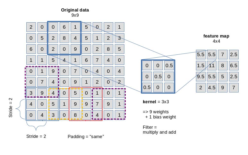
A “filter” defines a kind of masking pixel area of limited small size (e.g. 3×3 pixels). A filter combines weighted output values at neighboring nodes of a input layer in a specific defined way. It processes the offered information in a defined area always in the same fixed way –
independent of where the filter area is exactly placed on the (bigger) image (or a processed version of it). We call a processed version of an image a “map“.

A specific type of CNN layer, called a “Convolution Layer” [Conv layer], and a related operational algorithm let a series of such small masking areas cover the complete surface of an image (or a map). The first Conv layer of a CNN filters the information of the original image information via a multitude of such masking areas. The masks can be arranged overlapping, i.e. they can be shifted against each other by some distance along their axes. Think of the masking filter areas as a bunch of overlapping tiles covering the image. The shift is called stride.

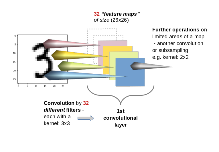
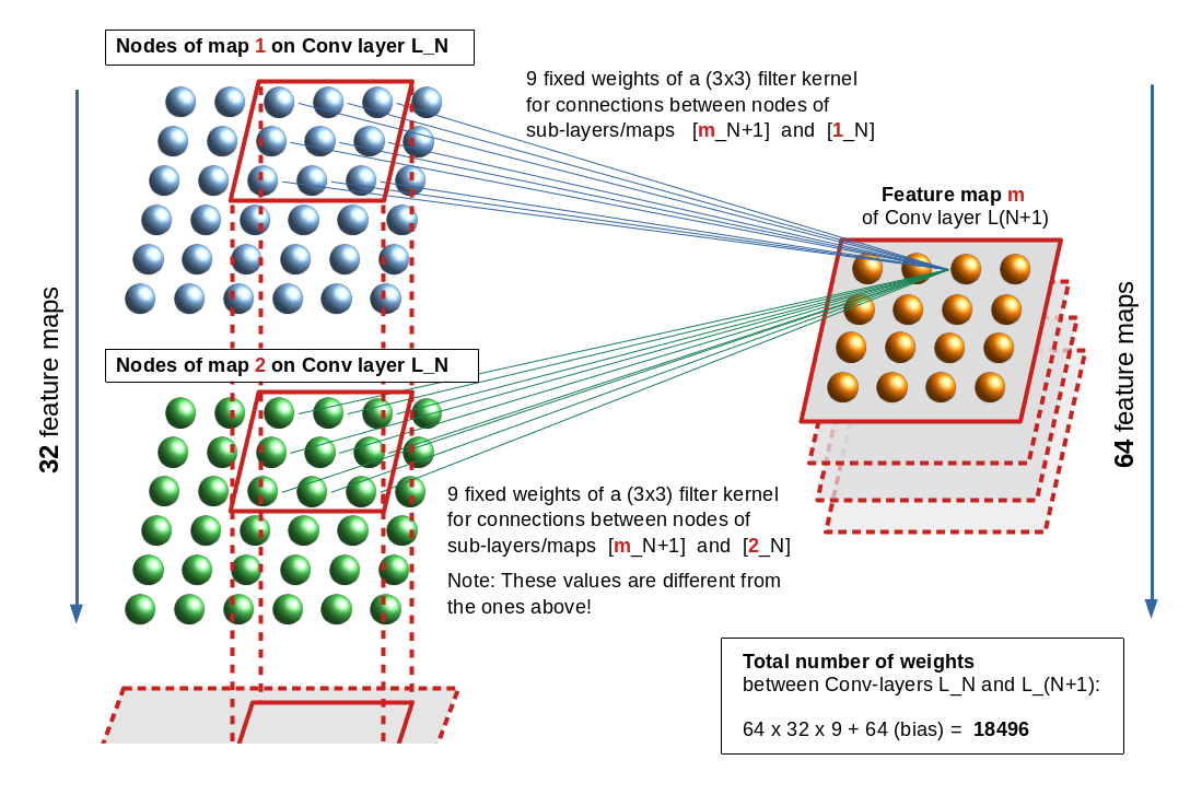
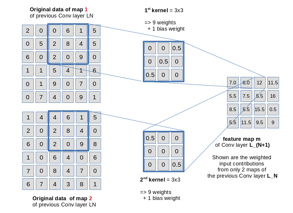
The “filter” mechanism (better: the mathematical recipe) of a specific filter remains the same for all of its small masking areas covering the image. A specific filter emphasizes certain parts of the original information and suppresses other parts in a defined way. If you combine the information of all masks you get a new (filtered) representation of the image – we speak of a “feature map” – sometimes with a smaller size than the original image (or map) the filter is applied to. The blending of the original data with a filtering mask creates a “feature map“, i.e. a filtered view onto the input data. The blending process is called “convolution” (due to the related mathematical operations).

The picture below sketches the basic principle of a 3×3-filter which is applied with a constant stride of 2 along each axis of the image:

Convolution is not so complicated as it sounds. It means: You multiply the original data values in the covered small area by factors defined in the filter’s kernel and add the resulting values up to get a a distinct value at a defined position inside the map. In the given example with a stride of 2 we get a resulting feature map of 4×4 out of a original 9×9 (image or map).

Note that a filter need not be defined as a square. It can have a rectangular (n x m) shape with (n, m) being integers. (In principle we could also think of other tile forms as e.g. hexagons – as long as they can seamlessly cover a defined plane. Interesting, although I have not seen a hexagon based CNN in the literature, yet).

A filter’s kernel defines factors used in the convolution operation – one for each of the (n x m) defined points in the filter area.

Note also that filters may have a “depth” property when they shall be applied to three-dimensional data sets; we may need a depth when we cover colored images (which require 3 input layers). But let us keep to flat filters in this introductory discussion …

Now we come to a central question: Does a CNN Conv layer use just one filter? The answer is: No!

A Conv layer of a CNN you allows for the construction of multiple different filters. Thus we have to deal with a whole bunch of filters per each convolutional layer. E.g. 32 filters for the first convolutional layer and 64 for the second and 128 for the third. The outcome of the respective filter operations is the creation is of equally many “feature maps” (one for each filter) per convolutional layer. With 32 different filters on a Conv layer we would thus build 32 maps at this layer.

This means: A Conv layer has a multitude of sub-layers, i.e. “maps” which result of the application of different filters on previous image or map data.

You may have guessed already that the next step of abstraction is:
You can apply filters also to “maps” of previous filters, i.e. you can chain convolutions. Thus, feature maps are either connected to the image (1st Conv layer) or to the maps of a previous layer.

By using a sequence of multiple Conv layers you cover growing areas of the original image. Everything clear? Probably not …

Filters and their related weights are the end products of the training and optimization of a CNN!

When I first was confronted with the concept of filters, I got confused because many authors only describe the basic technical details of the “convolution” mechanism. They explain with many words how a filter and its kernel work when the filtering area is “moved” across the surface of an image. They give you pretty concrete filter examples; very popular are straight lines and crosses indicated by “ones” as factors in the filter’s kernel and zeros otherwise. And then you get an additional lecture on strides and padding. You have certainly read various related passages in books about ML and/or CNNs. A pretty good example for this “explanation” is the (otherwise interesting and helpful!) book of Deru and Ndiaye (see the bottom of this article. I refer to the introductory chapter 3.5.1 on CNN architectures.)

Well, the technical procedure is pretty easy to understand from drawings as given above – the real question that nags in your brain is:

“Where the hell do all the different filter definitions come from?”

What many authors forget is a central introductory sentence for beginners:

A filter is not given a priori. Filters (and their kernels) are systematically constructed and build up during the training of a CNN; filters are the end products of a learning and optimization process every CNN must absolve.

This means: For a given problem or dataset you do not know in advance what the “filters” (and their defining kernels) will look like after training (aside of their pixel dimensions already fixed by the CNN’s layer definitions). The “factors” of a filter used in the convolution operation are actually weights, whose final values are the outcome of a learning process. Just as in MLPs …

Nothing is really “moved” …

Another critical point is the somewhat misleading analogy of “moving” a filter across an image’s or map’s pixel surface. Nothing is ever actually “moved” in a CNN’s algorithm. All masks are already in place when the convolution operations are performed:

Every element of a specific e.g. 3×3 kernel corresponds to “factors” for the convolution operation. What are these factors? Again: They are nothing else but weights – in exactly the same sense as we used them in MLPs. A filter kernel represents a set of weight-values to be multiplied with original output values at the “nodes” in other layers or maps feeding input to the nodes of the present map.

Things become much clearer if you imagine a feature map as a bunch of arranged “nodes”. Each node of a map is connected to (n x m) nodes of a previous set of nodes on a map or layer delivering input to the Conv layer’s maps.

Let us look at an example. The following drawing shows the connections from “nodes” of a feature map “m” of a Conv layer L_(N+1) to nodes of two different maps “1” and “2” of
Conv layer L_N. The stride for the kernels is assumed to be just 1.

In the example the related weights are described by two different (3×3) kernels. Note, however, that each node of a specific map uses the same weights for connections to another specific map or sub-layer of the previous (input) layer. This explains the total number of weights between two sequential Conv layers – one with 32 maps and the next with 64 maps – as (64 x 32 x 9) + 64 = 18496. The 64 extra weights account for bias values per map on layer L_(N+1). (As all nodes of a map use fixed bunches of weights, we only need exactly one bias value per map).

Note also that a stride is defined for the whole layer and not per map. Thus we enforce the same size of all maps in a layer. The convolutions between a distinct map and all maps of the previous layer L_N can be thought as operations performed on a column of stacked filter areas at the same position – one above the other across all maps of L_N. See the illustration below:

The weights of a specific kernel work together as an ensemble: They condense the original 3×3 pixel information in the filtered area of the connected input layer or a map to a value at one node of the filter specific feature map. Please note that there is a bias weight in addition for every map; however, at all masking areas of a specific filter the very same 9 weights are applied. See the next drawing for an illustration of the weight application in our example for fictitious node and kernel values.

A CNN learns the appropriate weights (= the filter definitions) for a given bunch of images via training and is guided by the optimization of a loss function. You know these concepts already from MLPs …

The difference is that the ANN now learns about appropriate “weight ensembles” – eventually (!) working together as a defined convolutional filter between different maps of neighboring Conv (and/or sampling ) Layers. (For sampling see a separate paragraph below.)

The next picture illustrates the column like convolution of information across the identically positioned filter areas across multiple maps of a previous convolution layer:

The fact that the weight ensemble of a specific filter between maps is always the same, explains, by the way, the relatively (!) small number of weight parameters in deep CNNS.

Intermediate summary: The weights, which represent the factors used by a specific filter operation called convolution, are defined during a training process. The filter, its kernel and the respective weight values are the outcome of a mathematical optimization process – mostly guided by gradient descent.

Activation functions

As in MLPs each Conv layer has an associated “activation function” which is applied at each node of all maps after the resulting values of the convolution have been calculated as
the nodes input. The output then feeds the connections to the next layer. In CNNs for image handling often “Relu” or “Selu” are used as activation functions – and not “sigmoid” which we applied in the MLP code discussed in another article series of this blog.

Tensors

The above drawings indicate already that we need to arrange the data (of an image) and also the resulting map data in an organized way to be able to apply the required convolutional multiplications and summations the right way.

An colored image is basically a regular 3 dimensional structure with a width “w” (number of pixels along the x-axis), a height “h” (number of pixels along the y-axis) and a (color) depth “d” (d=3 for RGB colors).

If you represent the color value at each pixel and RGB-layer by a float you get a bunch of w x h x d float values which we can organize and index in a 3 dimensional Numpy array. Mathematically such well organized arrays with a defined number of axes (rank), a set of numbers describing the dimension along each axis (shape), a data-type, possible operations (and invariance aspects) define an abstract object called a “tensor“. Colored image data can be arranged in 3-dimensional tensors; gray colored images in a pseudo 3D-tensor which has a shape of (n, m, 1). (Keras and Tensorflow want to get imagedata in form of 2D tensors).

Now the important point is: The output data of Conv-layers and their feature maps also represent tensors. A bunch of 32 maps with a defined width and height defines data of a 3D-tensor.

You can imagine each value of such a tensor as the input or output given at a specific node in a layer with a 3-dimensional sub-structure. (In other even more complex data structures than images we would other multi-dimensional data structures.) The weights of a filter kernel describe the connections of the nodes of a feature map on a layer L_N to a specific map of a previous layer. Weights, actually, also define elements of a tensor.

The forward- and backward-propagation operations performed throughout such a complex net during training thus correspond to sequences of tensor-operations – i.e. generalized versions of the np.dot()-product we got to know in MLPs.

You understood already that e.g strides are important. But you do not need to care about details – Keras and Tensorflow will do the job for you! If you want to read a bit look a the documentation of the TF function “tf.nn.conv2d()”.

When we later on train with mini-batches of input data (i.e. batches of images) we get yet another dimension of our tensors. This batch dimension can – quite similar to MLPs – be used to optimize the tensor operations in a vectorized way. See my series on MLPs.

Chained convolutions cover growing areas of the original image

Two sections above I characterized the training of a CNN as a two-fold procedure. From the first drawing it is relatively easy to understand how we get to grasp tiny sub-structures of an image: Just use filters with small kernel sizes!

Fine, but there is probably a second question already arising in your mind:

By what mechanism does a CNN find or recognize a hierarchy of features?

One part of the answer is: Chain convolutions!

Let us assume a first convolutional layer with filters having a stride of 1 and a (3×3) kernel. We get maps with a shape of (26, 26) on this layer. The next Conv layer shall use a (4×4) kernel and also a stride of 1; then we get maps with a shape of (23, 23). A node on the second layer covers (6×6)-arrays on the original image. Two neighboring nodes a total area of (7×7). The individual (6×6)-areas of course overlap.

With a stride of 2 on each Conv-layer the corresponding areas on the original image are (7×7) and (11×11).

So a stack of consecutive (sequential) Conv-layers covers growing areas on the original image. This supports the detection of a pattern or feature hierarchy in the data of the input images.

However: Small strides require a relatively big number of sequential Conv-layers (for 3×3 kernels and stride 2) at least 13 layers to eventually cover the full image area.

Even if we would not enlarge the number of maps beyond 128 with growing layer number, we would get

(32 x 9 + 32) + (64 x 32 +64) + (128 x 64 + 128) + 10 x (128 x 128 + 128) = 320 + 18496 + 73856 + 10*147584 = 1.568 million weight parameters

to take care of!

This number has to be multiplied by the number of images in a mini-batch – e.g. 500. And – as we know from MLPs we have to keep all intermediate output results in RAM to accelerate the BW propagation for the determination of gradients. Too many data and parameters for the analysis of small 28×28 images!

Big strides, however, would affect the spatial resolution of the first layers in a CNN. What is the way out?

Sub-sampling is necessary!

The famous VGG16 CNN uses pairs and triples of convolution chains in its architecture. How does such a network get control over the number of weight parameters and the RAM requirement for all the output data at all the layers?

To get information in the sense of a feature hierarchy the CNN clearly should not look at details and related small sub-fields of the image, only. It must cover step-wise growing (!) areas of the original image, too. How do we combine these seemingly contradictory objectives in one training algorithm which does not lead to an exploding number of parameters, RAM and CPU time? Well, guys, this is the point where we should pay due respect to all the creative inventors of CNNs:

The answer is: We must accumulate or sample information across larger image or map areas. This is the (underestimated?) task of pooling– or sampling-layers.

For me it was just another confusing point in the beginning – until one grasps the real magic behind it. At first sight a layer like a typical “maxpooling” layer seems to reduce information, only; see the next picture:

The drawing explains that we “sample” the information over multiple pixels e.g. by

  • either calculating an average over pixels (or map node values)
  • or by just picking the maximum value of pixels or map node values (thereby stressing the most important information)

in a certain defined sub-area of an image or map.

The shift or stride used as a default in a pooling layer is exactly the side length of the pooling area. We thus cover the image by adjacent, non-overlapping tiles! This leads to a substantial decrease of the dimensions of the resulting map! With a (2×2) pooling size by a an effective factor of 2. (You can change the default pooling stride – but think about the consequences!)

Of course, averaging or picking a max value corresponds to information reduction.

However: What the CNN really also will do in a subsequent Conv layer is to invest in further weights for the combination of information (features) in and of substantially larger areas of the original image! Pooling followed by an additional convolution obviously supports hierarchy building of information on different scales of image areas!

After we first have concentrated on small scale features (like with a magnifying glass) we now – in a figurative sense – make a step backwards and look at larger scales of the image again.

The trick is to evaluate large scale information by sampling layers in addition to the small scale information information already extracted by the previous convolutions. Yes, we drop resolution information – but by introducing a suitable mix of convolutions and sampling layers we also force the network systematically to concentrate on combined large scale features, which in the end are really important for the image classification as a whole!

As sampling counterbalances an explosion of parameters we can invest into a growing number of feature maps with growing scales of covered image areas. I.e. we add more and new filters reacting to combinations of larger scale information.

Look at the second to last illustration: Assume that the 32 maps on layer L_N depicted there are the result of a sampling operation. The next convolution gathers new knowledge about more, namely 64 different combinations of filtered structures over a whole vertical stack of small filter areas located at the same position on the 32 maps of layer N. The new information is in the course of training conserved into 64 weight ensembles for 64 maps on layer N+1.

Resulting options for architectures

We can think of multiple ways of combining Conv layers and pooling layers. A simple recipe for small images could be

  • Layer 0: Input layer (tensor of original image data, 3 color layers or one gray layer)
  • Layer 1: Conv layer (small 3×3 kernel, stride 1, 32 filters, 32 maps (26×26), analyzes 3×3 overlapping areas)
  • Layer 2: Pooling layer (2×2 max pooling => 32 (13×13) maps,
    a node covers 4×4 non overlapping areas per node on the original image)
  • Layer 3: Conv layer (3×3 kernel, stride 1, 64 filters, 64 maps (11×11),
    a node covers 8×8 overlapping areas on the original image (total effective stride 2))
  • Layer 4: Pooling layer (2×2 max pooling => 64 maps (5×5),
    a node covers 10×10 areas per node on the original image (total effective stride 5), some border info lost)
  • Layer 5: Conv layer (3×3 kernel, stride 1, 64 filters, 64 maps (3×3),
    a node covers 18×18 per node (effective stride 5), some border info lost )

The following picture illustrates the resulting successive combinations of nodes along one axis of a 28×28 image.

Note that I only indicated the connections to border nodes of the Conv filter areas.

The kernel size decides on the smallest structures we look at – especially via the first convolution. The sampling decides on the sequence of steadily growing areas which we then analyze for specific combinations of smaller structures.

Again: It is most of all the (down-) sampling which allows for an effective hierarchical information building over growing larger image areas! Actually we do not really drop information by sampling – instead we give the network a chance to collect and code new information on a higher, more abstract level (via a whole bunch of numerous new weights).

The big advantages of the sampling layers get obvious:

  • They reduce the numbers of required weights
  • They reduce the amount of required memory – not only for weights but also for the output data, which must be saved for every layer, map and node.
  • They reduce the CPU load for FW and BW propagation
  • They also limit the risk of overfitting as some detail information is dropped.

Of course there are many other sequences of layers one could think about. E.g., we could combine 2 to 3 Conv layers before we apply a pooling layer. Such a layer sequence is characteristic of the VGG nets.

Further aspects

Just as MLPs a CNN represents an acyclic graph, where the maps contain increasingly fewer nodes but where the number of maps per layer increases on average.

Questions and objectives for this article series

An interesting question, which seldom is answered in introductory books, is whether two totally independent training runs for a given CNN-architecture applied on the same input data will produce the same filters in the same order. We shall investigate this point in the forthcoming articles.

Another interesting point is: What does a CNN see at which convolution layer?
And even more important: What do the “features” (= basic structural elements) in an image which trigger/activate a specific filter or map, look like?

If we could look into the output at some maps we could possibly see what filters do with the original image. And if we found a way to construct a structured image which triggers a specific filter then we could better understand what patterns the CNN reacts to. Are these patterns really “features” in the sense of conceptual entities? Examples for these different types of visualizations with respect to convolution in a CNN are objectives of this article series.

Conclusion

Today we covered a lot of “theory” on some aspects of CNNs. But we have a sufficiently solid basis regarding the structure and architecture now.

CNNs obviously have a much more complex structure than MLPs: They are deep in the sense of many sequential layers. And each convolutional layer has a complex structure in form of many parallel sub-layers (feature maps) itself. Feature maps are associated with filters, whose parameters (weights) get learned during the training. A map results from covering the original image or a map of a previous layer with small (overlapping) tiles of small filtering areas.

A mix of convolution and pooling layers allows for a look at detail patterns of the image in small areas in lower layers, whilst later layers can focus on feature combinations of larger image areas. The involved filters thus allow for the “awareness” of a hierarchy of features with translational invariance.

Pooling layers are important because they help to control the amount of weight parameters – and they enhance the effectiveness of detecting the most important feature correlations on larger image scales.

All nice and convincing – but the attentive reader will ask: Where and how do we do the classification?
Try to answer this question yourself first.

In the next article we shall build a concrete CNN and apply it to the MNIST dataset of images of handwritten digits. And whilst we do it I deliver the answer to the question posed above. Stay tuned …

Literature

“Advanced Machine Learning with Python”, John Hearty, 2016, Packt Publishing – See chapter 4.

“Deep Learning mit Python und Keras”, Francois Chollet, 2018, mitp Verlag – See chapter 5.

“Hands-On Machine learning with SciKit-Learn, Keras & Tensorflow”, 2nd edition, Aurelien Geron, 2019, O’Reilly – See chapter 14.

“Deep Learning mit Tensorflow, keras und Tensorflow.js”, Matthieu Deru, Alassane Ndiaye, 2019, Rheinwerk Verlag, Bonn – see chapter 3

Further articles in this series

A simple CNN for the MNIST dataset – XI – Python code for filter visualization and OIP detection
A simple CNN for the MNIST dataset – X – filling some gaps in filter
visualization

A simple CNN for the MNIST dataset – IX – filter visualization at a convolutional layer
A simple CNN for the MNIST dataset – VIII – filters and features – Python code to visualize patterns which activate a map strongly
A simple CNN for the MNIST dataset – VII – outline of steps to visualize image patterns which trigger filter maps
A simple CNN for the MNIST dataset – VI – classification by activation patterns and the role of the CNN’s MLP part
A simple CNN for the MNIST dataset – V – about the difference of activation patterns and features
A simple CNN for the MNIST dataset – IV – Visualizing the activation output of convolutional layers and maps
A simple CNN for the MNIST dataset – III – inclusion of a learning-rate scheduler, momentum and a L2-regularizer
A simple CNN for the MNIST datasets – II – building the CNN with Keras and a first test
A simple CNN for the MNIST datasets – I – CNN basics

Addendum 20.10.2020: “Feature maps” or “response maps”?

Whilst reading some more books on AI I got the impression that some authors associate the term “feature map” with the full collection of all maps related to a Conv layer. A single map then is called a “response map” or an “output channel” of the feature map. However, as most books (e.g. the book of A. Geron on Machine Learning) call a singular map a “feature map” I cling to this usage throughout this series.